CONTENT OF THE MARKET PATTERNS DASHBOARD PAGES
Price & Volume Highlights
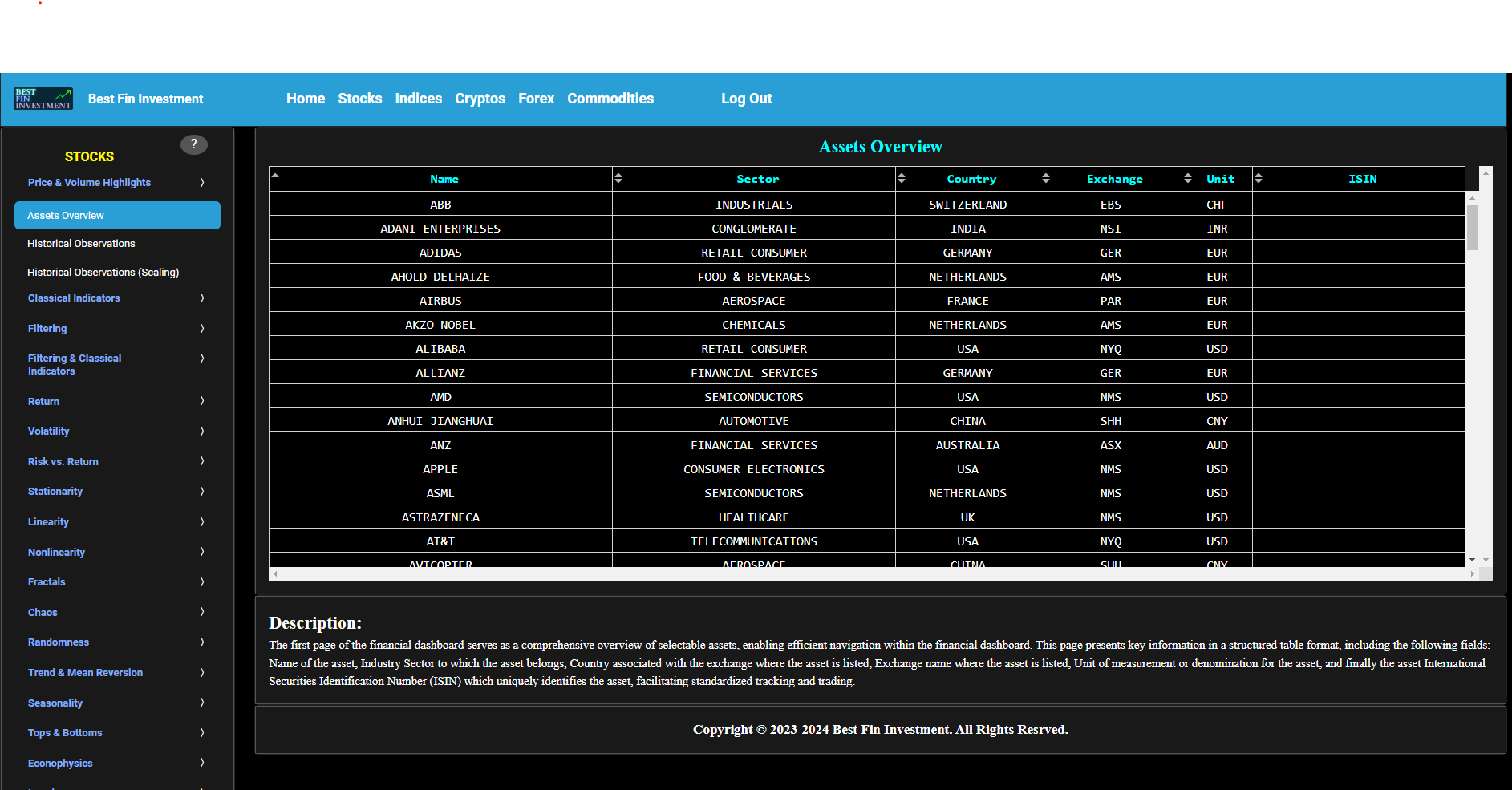
Assets Overview
This first page of the market patterns dashboard serves as a comprehensive overview of selectable assets, enabling efficient navigation within the dashboard's subsequent pages. The current page presents key information in a structured table format, including the following fields: name of the asset, asset ticker, country associated with the exchange where the asset is listed, industry sector to which the asset belongs, exchange name where the asset is listed, and unit of measurement or denomination for the asset.
Price & Volume Highlights
Historical Observations
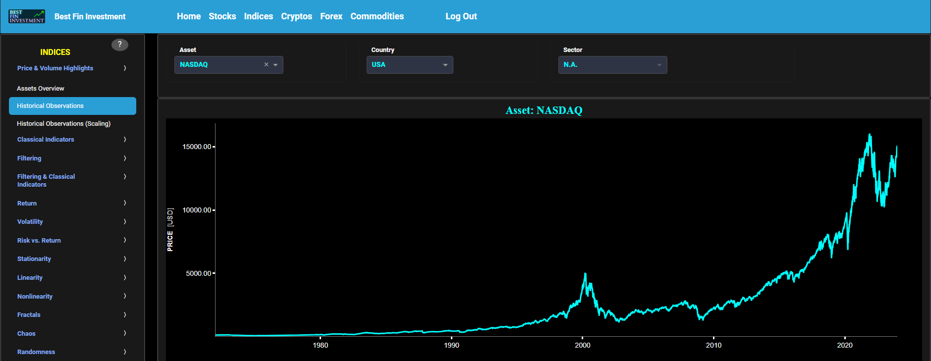
This page visualizes the full historical data range of a selected asset, based upon daily close prices. In the menu bar (located just above the graphs), you can also see the associated asset country and asset sector (wherever applicable). A price and volume graph will appear after the selection of an asset, or the selection of a country followed by the selection of an available asset within that country.
Price & Volume Highlights
Historical Observations (Scaling)
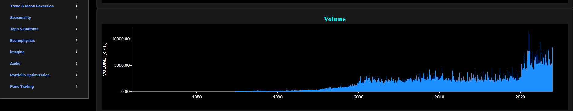
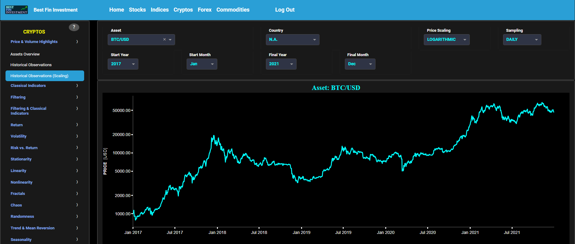
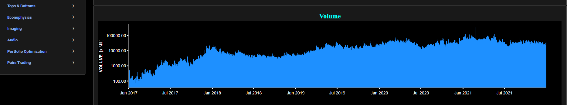
This page visualizes historical asset prices and volume using either daily, weekly, or monthly close prices. In the menu bar (located just above the graphs), you can also see (and select) the associated asset country. Further you can select specific time periods to visualize and also toggle between a linear or logarithmic price and volume scaling on the y-axis.
Classical Indicators
Candlesticks
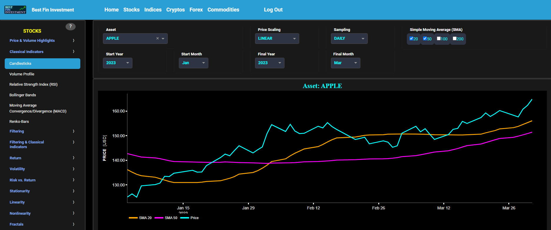
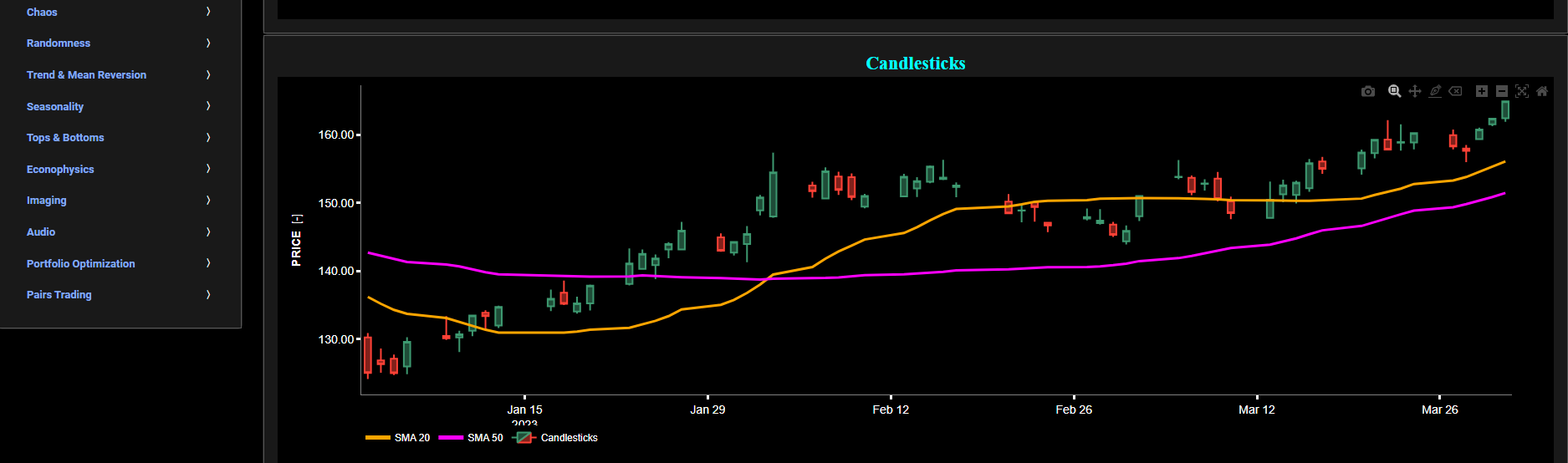
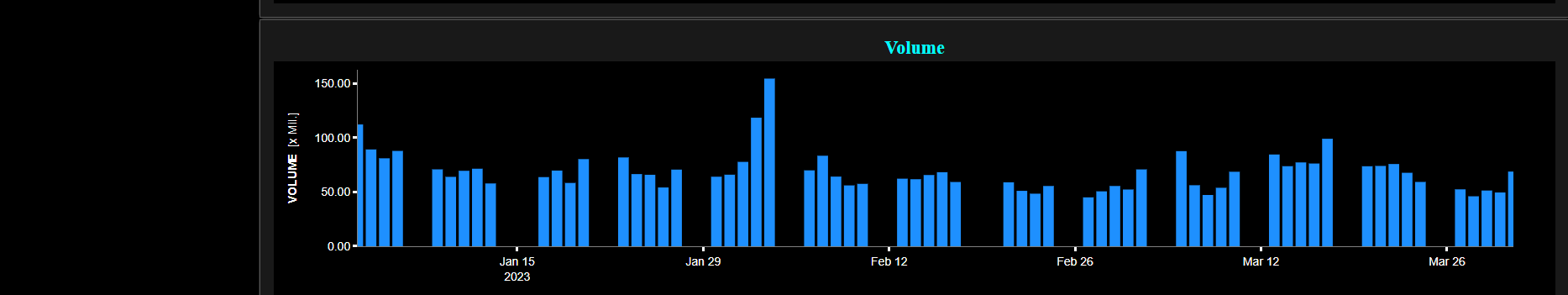
This page provides 3 graphs. The upper graph visualizes historical asset prices using either daily, weekly, or monthly close prices. In the menu bar (located just above the graphs), you can also select specific time periods to visualize and also toggle between a linear or logarithmic price scaling on the y-axis. In addition the upper graph allows you to superimpose several Simple Moving Average (SMA) lines. The middle graph shows the corresponding candlesticks visualization, whereas the lower graph presents the volume indicator for the selected asset.
Classical Indicators
Volume Profile
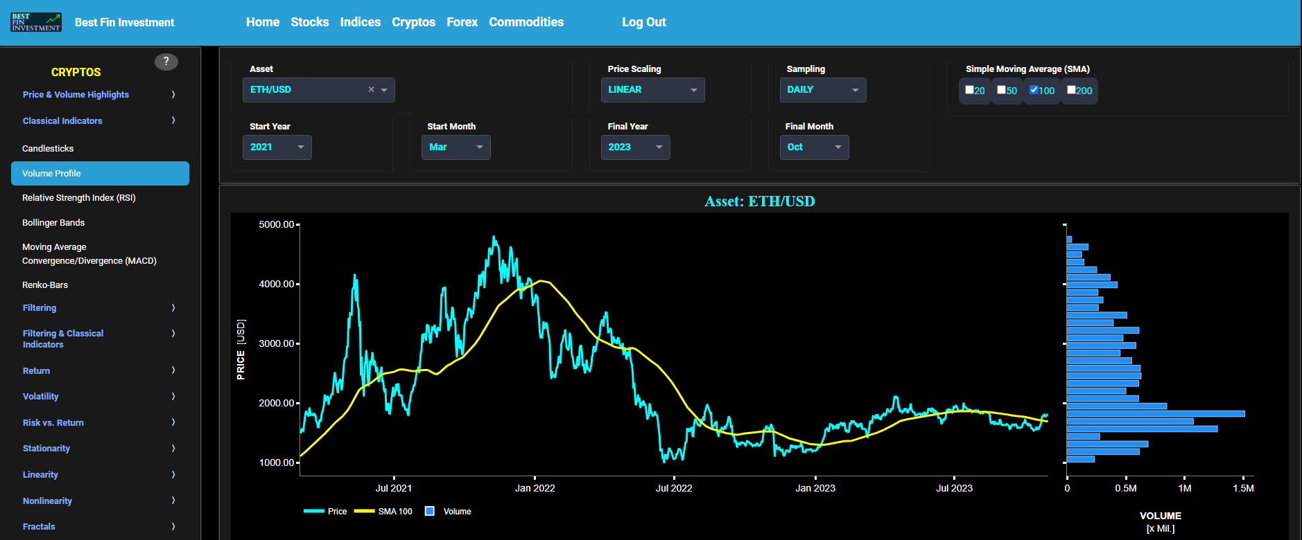
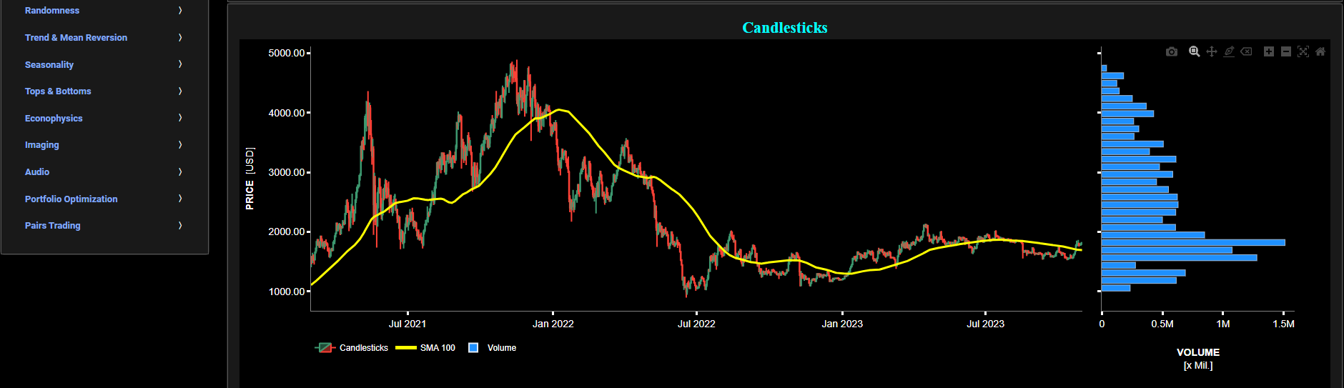
This page provides 2 graphs. The upper graph visualizes historical asset prices using either daily, weekly, or monthly close prices. In the menu bar (located just above the graphs), you can also select specific time periods to visualize and also toggle between a linear or logarithmic price scaling on the y-axis. In addition the upper graph allows you to superimpose several Simple Moving Average (SMA) lines. Next the right-side of the upper graph shows the so-called Volume Profile chart, i.e. the volume histogram (bar graph) which represents the distribution of volume at each price level over a specific time period. This allows to visualize where the majority of trading activity occurred and may be useful to identify support and resistance levels based on volume distribution at various price levels. The lower graph shows the corresponding candlesticks visualization with its associated Volume Profile chart.
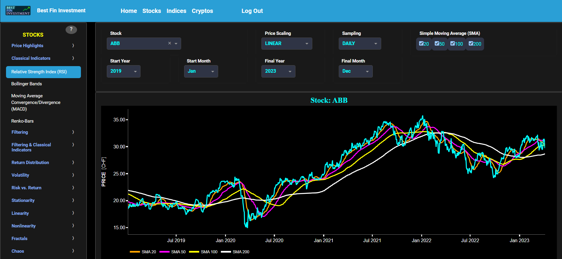
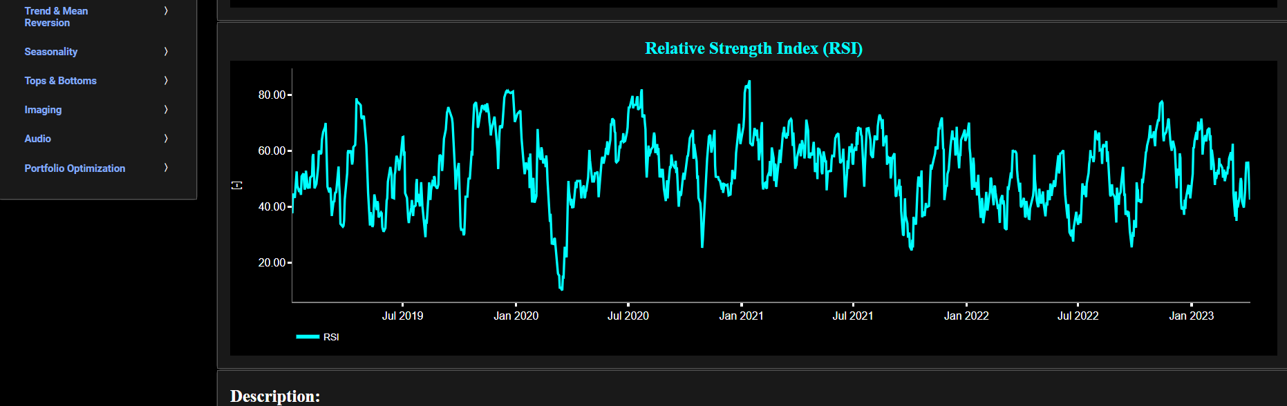
Classical Indicators
Relative Strength Index (RSI)
This page provides 2 graphs. The upper graph visualizes historical asset prices using either daily, weekly, or monthly close prices. In the menu bar (located just above the graphs), you can also select specific time periods to visualize and also toggle between a linear or logarithmic price scaling on the y-axis. In addition the upper graph allows you to superimpose several Simple Moving Average (SMA) lines. The lower graph presents the standard 14-period Relative Strength Index (RSI) indicator for the selected asset price data.
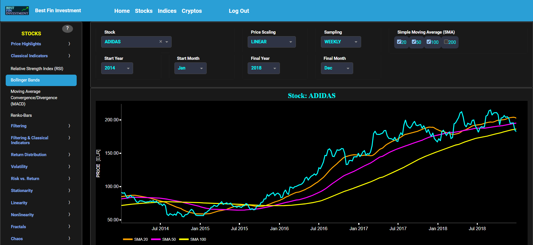
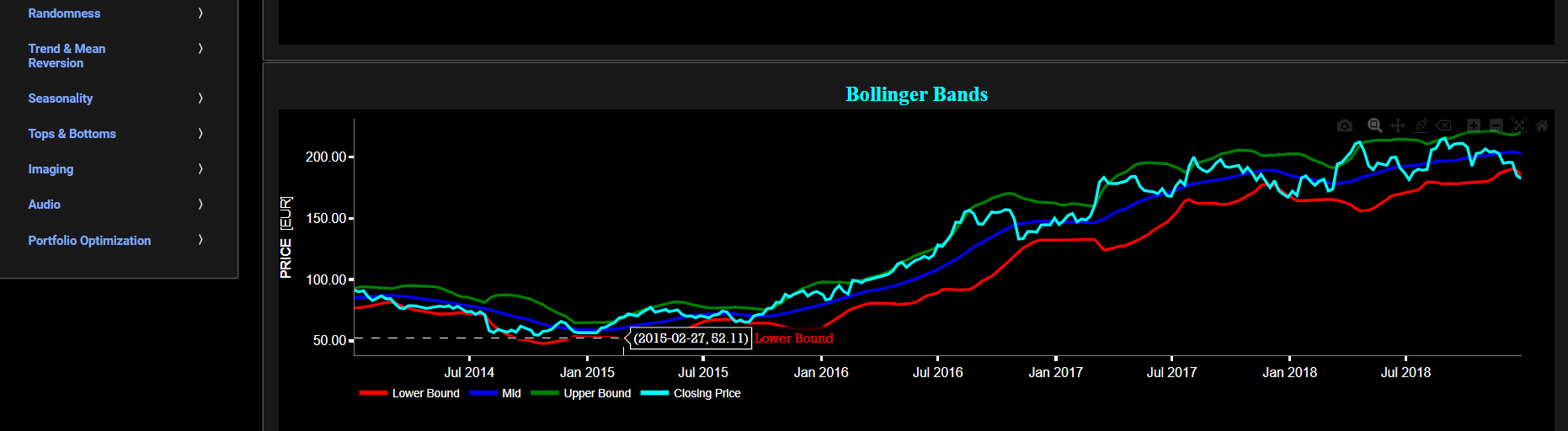
Classical Indicators
Bollinger Bands
This page provides 2 graphs. The upper graph visualizes historical asset prices using either daily, weekly, or monthly close prices. In the menu bar (located just above the graphs), you can also select specific time periods to visualize and also toggle between a linear or logarithmic price scaling on the y-axis. In addition the upper graph allows you to superimpose several Simple Moving Average (SMA) lines. The lower graph presents the Bollinger Bands indicator (computed on the basis of a standard 20-period moving average) for the selected asset price data.
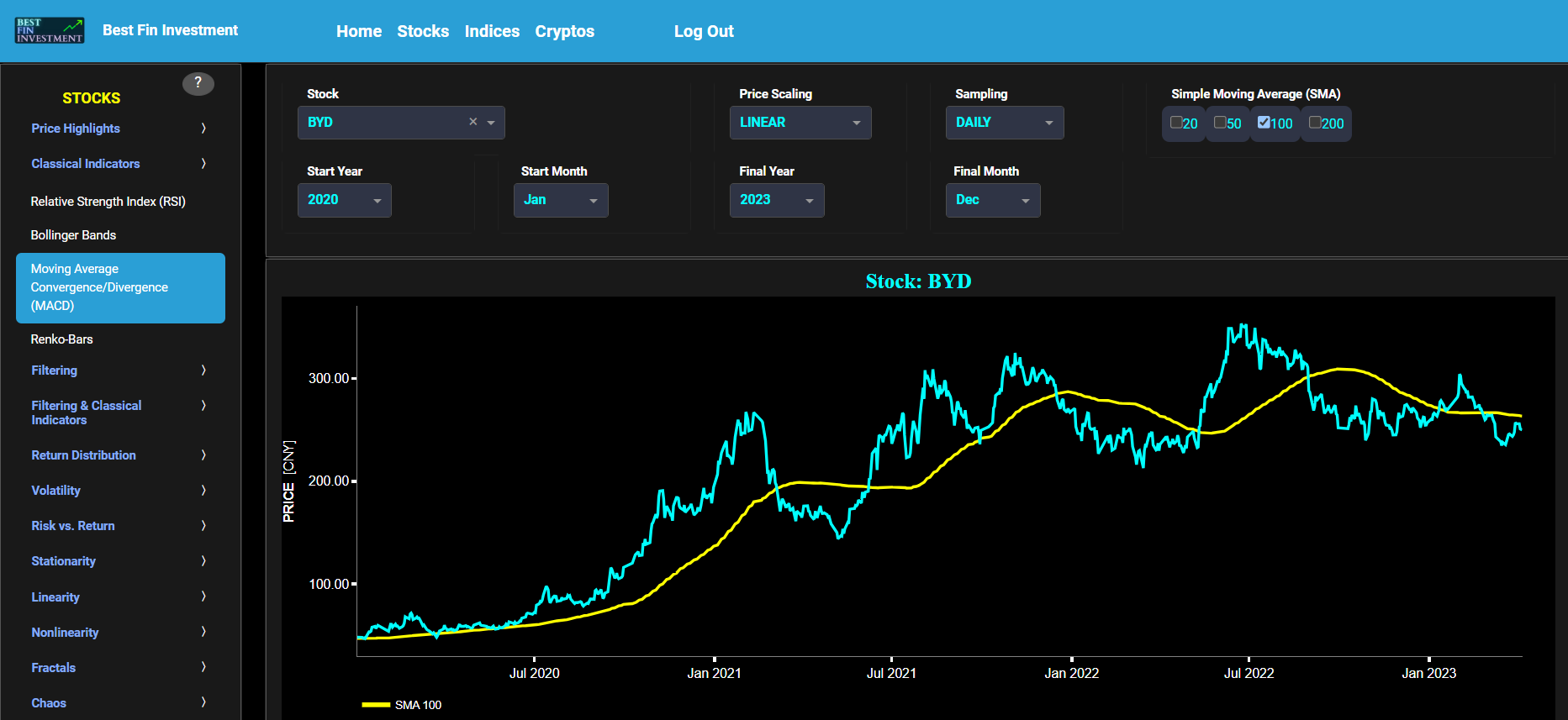
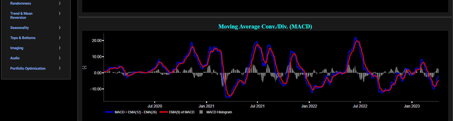
Classical Indicators
Moving Average Convergence/Divergence (MACD)
This page provides 2 graphs. The upper graph visualizes historical asset prices using either daily, weekly, or monthly close prices. In the menu bar (located just above the graphs), you can also select specific time periods to visualize and also toggle between a linear or logarithmic price scaling on the y-axis. In addition the upper graph allows you to superimpose several Simple Moving Average (SMA) lines. The lower graph presents the Moving Average Convergence/Divergence (MACD) indicator (using the standard 12,26,9 moving average periods) for the selected asset price data.
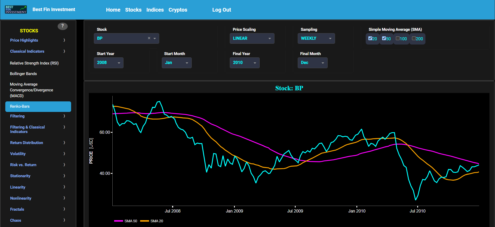
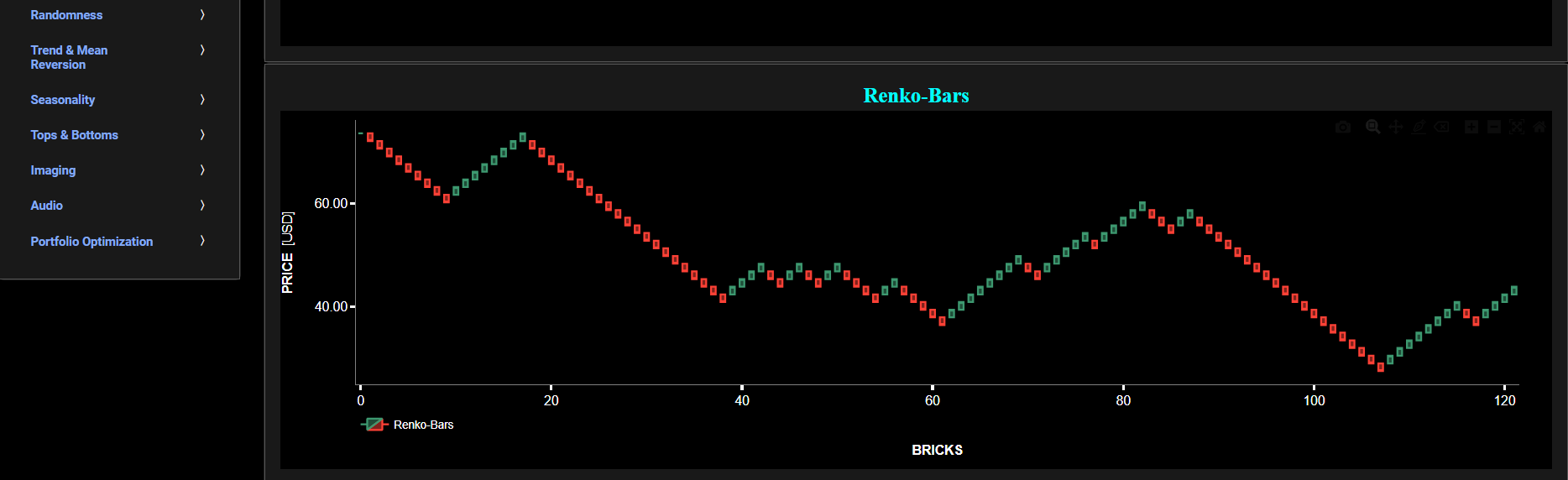
Classical Indicators
Renko-Bars
This page provides 2 graphs. The upper graph visualizes historical asset prices using either daily, weekly, or monthly close prices. In the menu bar (located just above the graphs), you can also select specific time periods to visualize and also toggle between a linear or logarithmic price scaling on the y-axis. In addition the upper graph allows you to superimpose several Simple Moving Average (SMA) lines. The lower graph presents the Renko Candle Bars indicator, using a simplified Average True Range (ATR) indicator, for the selected asset price data.
Filtering
Frequency Analysis
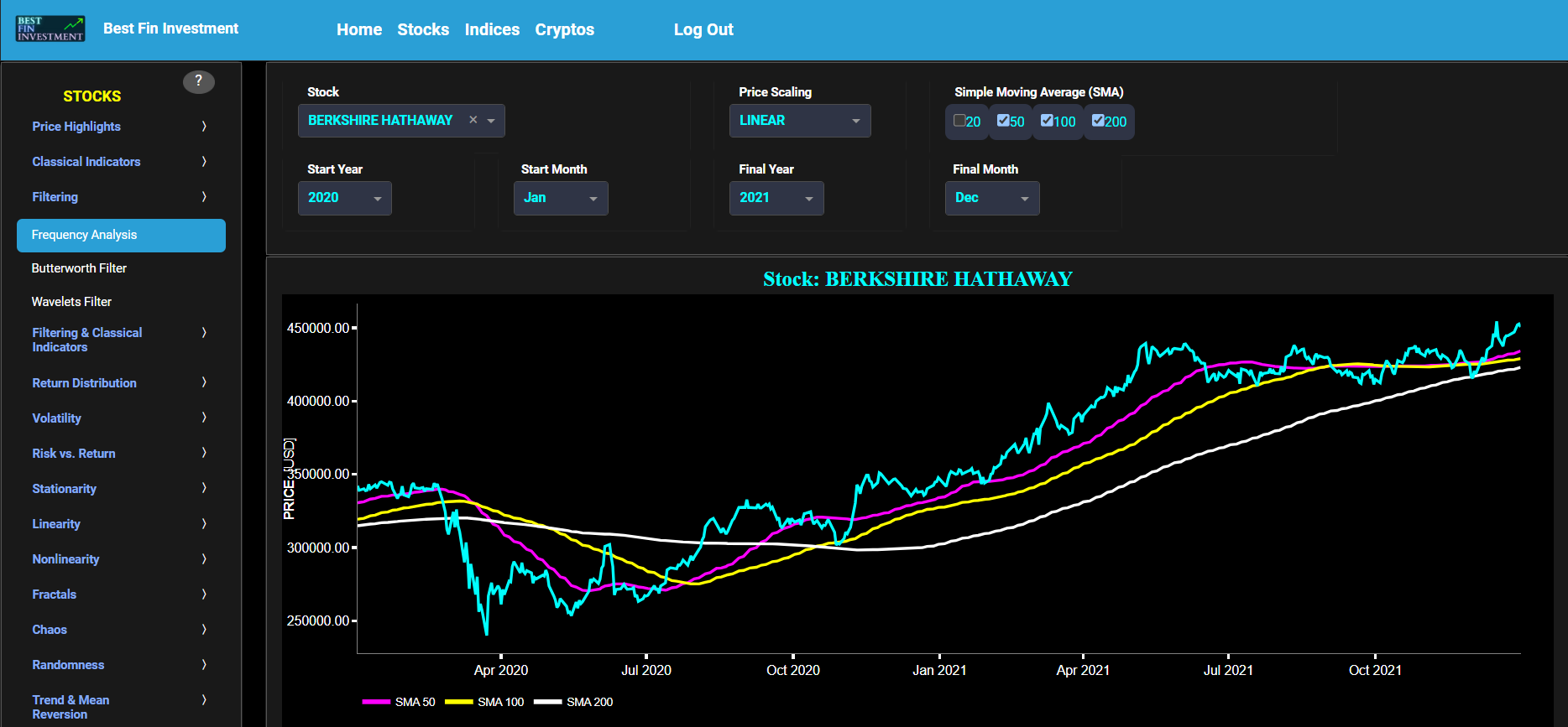
This page provides 2 graphs. The upper graph visualizes historical asset prices using either daily, weekly, or monthly close prices. In the menu bar (located just above the graphs), you can also select specific time periods to visualize and also toggle between a linear or logarithmic price scaling on the y-axis. In addition the upper graph allows you to superimpose several Simple Moving Average (SMA) lines.
The lower graph presents the frequency content of the price signal, computed through Fast Fourier Transform (FFT). For the lower graph x-axis unit we chose a more recognizable time period unit (expressed in Days) rather than the typical Herz metric. Beneath the lower graph there is a horizontal sliding bar which allows to select the cut-off time period (Tc, with Tc expressed in Days) of a low-pass filter. The purpose of such a filter would be to smoothen-out the original price signal, i.e. by filtering out (or removing) any high-frequency content (with frequency > 1/Tc), or equivalently, by removing the low-periodic signal content (with period < Tc). The green background color of the lower graph essentially represents the price signal-content which would be preserved, after the application of this low-pass filter. This cut-off period (Tc) will subsequently be used within the page “Butterworth Filter” to perform a low-pass Butterworth filtering.
Filtering
Butterworth Filter
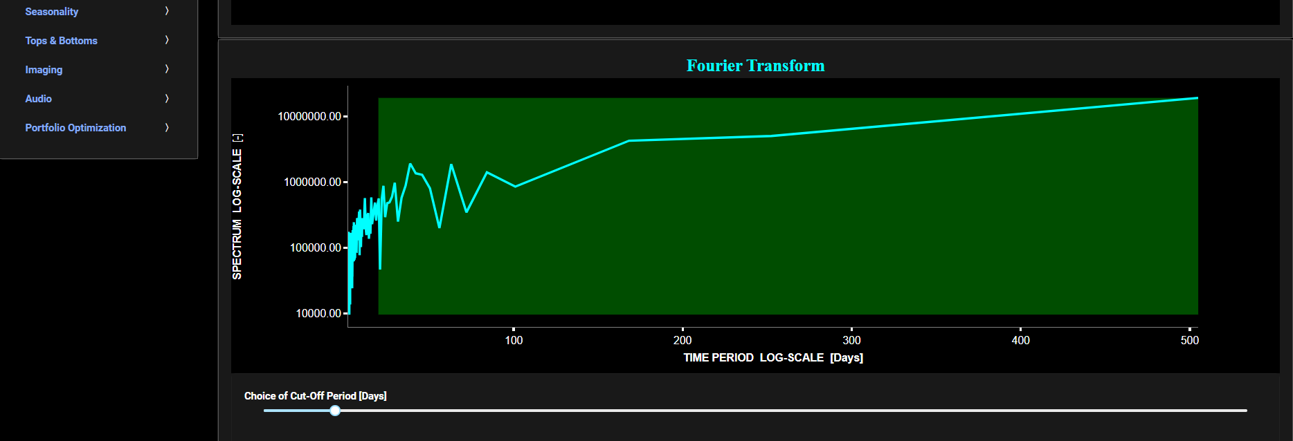
This page visualizes historical asset prices using daily close prices. In the menu bar (located just above the graph), you can also select specific time periods to visualize and also toggle between a linear or logarithmic price scaling on the y-axis. In addition the graph allows you to superimpose several Simple Moving Average (SMA) lines. Next this page allows you to add a filtered price signal obtained through the application of a low-pass Butterworth digital filter. Note that here we use a causal implementation of the filter, meaning that the filter output at time t is only influenced by data points up to time t. The filter cut-off time period (Tc), with Tc expressed in Days, can also be selected in the menu bar. The purpose of this filter is to smoothen-out the original price signal, i.e. by filtering out (or removing) any high-frequency content (with frequency > 1/Tc), or equivalently, by removing the low-periodic signal content (with period < Tc). Refer also to the lower graph on page "Frequency Analysis" to help you select an appropriate cut-off time period value.
Butterworth filters are widely employed across various engineering disciplines, including aerospace, electrical, and mechanical engineering, to effectively filter and process digital signals. Further you can also compare the results obtained with this Butterworth filter with the ones obtained using a Wavelet filter on page “Wavelets Filter”. Finally, this filter will be used within the pages located under section “Filtering & Classical Indicators” to first filter out the price signal data before applying one of the classical indicators.
Filtering
Wavelets Filter
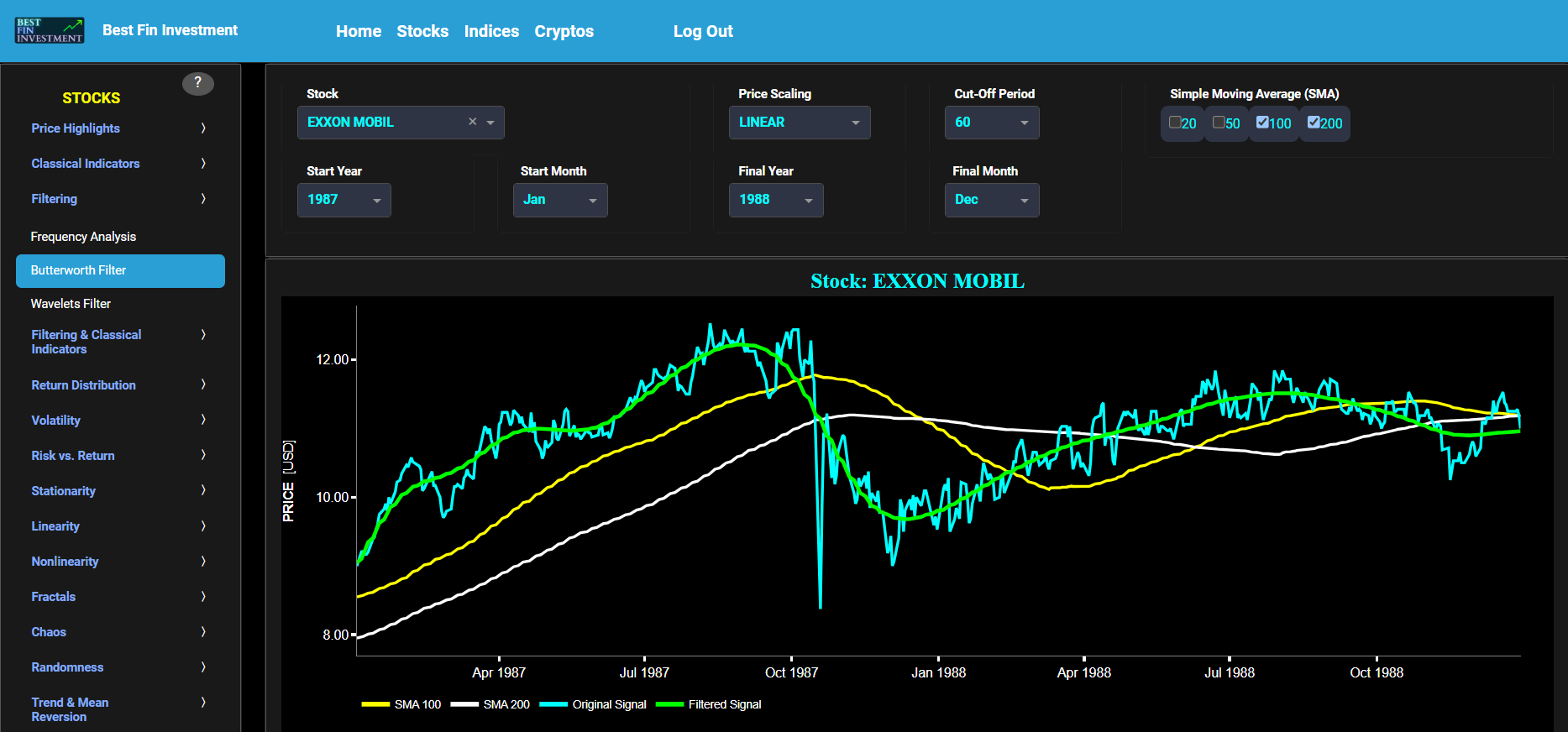
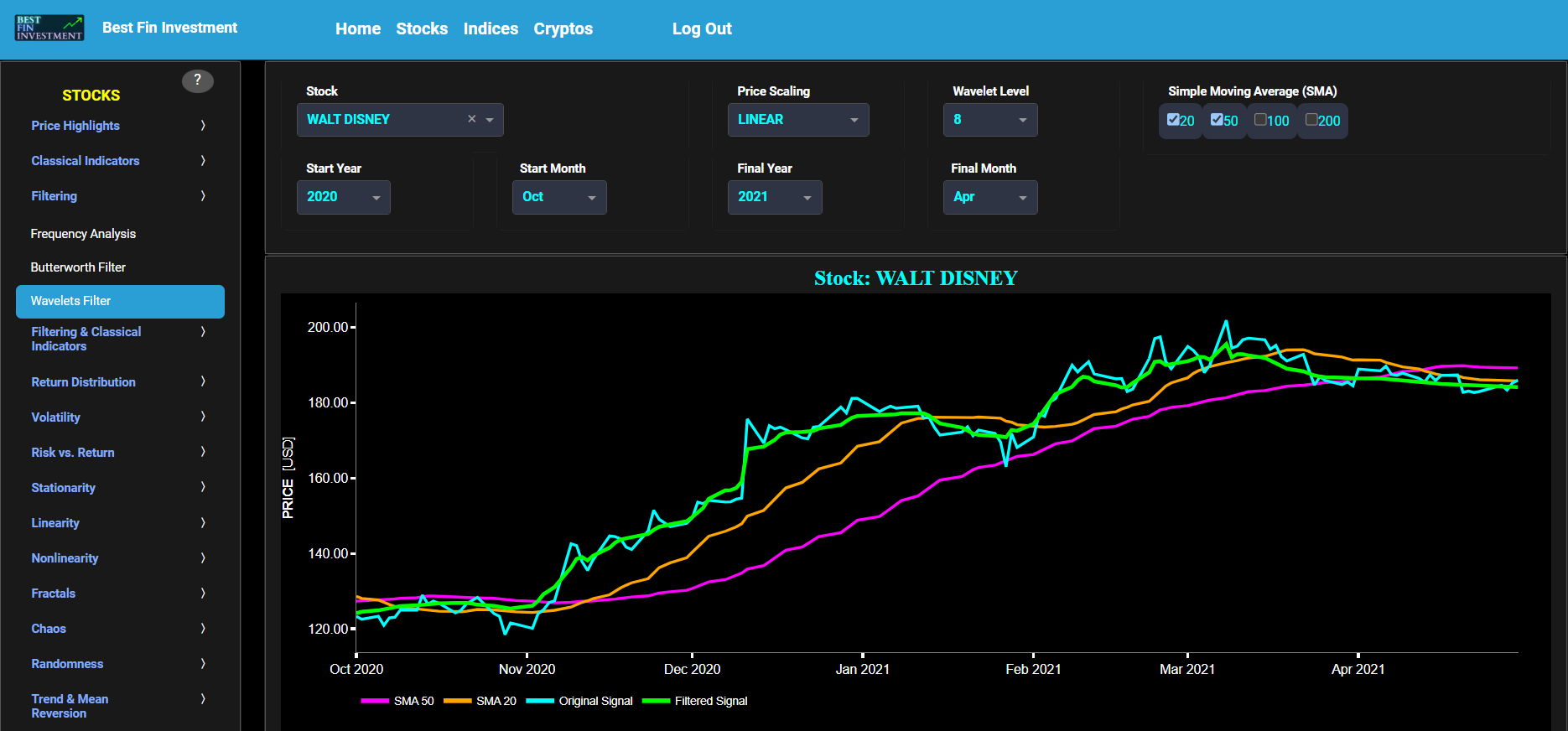
This page visualizes historical asset prices using daily close prices. In the menu bar (located just above the graph), you can also select specific time periods to visualize and also toggle between a linear or logarithmic price scaling on the y-axis. In addition the graph allows you to superimpose several Simple Moving Average (SMA) lines. Next this page allows you to add a filtered price signal obtained through the application of a Wavelet-based denoising filter. Please be aware that, unlike the Butterworth filter implementations used on other Dashboard pages, the current wavelet filter applied here is non-causal. This means the filter's output depends on both past and future data points, which can lead to potentially misleading or overly optimistic results, especially in real-time processing scenarios such as filtering daily asset prices. This non-causal filter is employed because standard wavelet functions are typically non-causal. However, after conducting tests using daily data, we have observed that the impact is not significant. Here we have used the "sym" (symmetric) wavelet family which tends to have good time-frequency localization properties and hence may be better suited for denoising non-stationary financial price data. The so-called Wavelet filter decomposition level can also be selected in the menu bar. The purpose of this filter is to smoothen-out the original price signal, i.e. by filtering out (or removing) any high-frequency content of the price signal.
Wavelet-based denoising filters are widely employed across various engineering disciplines, including aerospace, electrical, and mechanical engineering, to effectively filter and process digital signals. Further you can also compare the results obtained with this Wavelet filter with the ones obtained using a Butterworth filter on page “Butterworth Filter”. Finally, this filter will be used within the pages located under section “Filtering & Classical Indicators” to first filter out the price signal data before applying one of the classical indicators.
Filtering & Classical Indicators
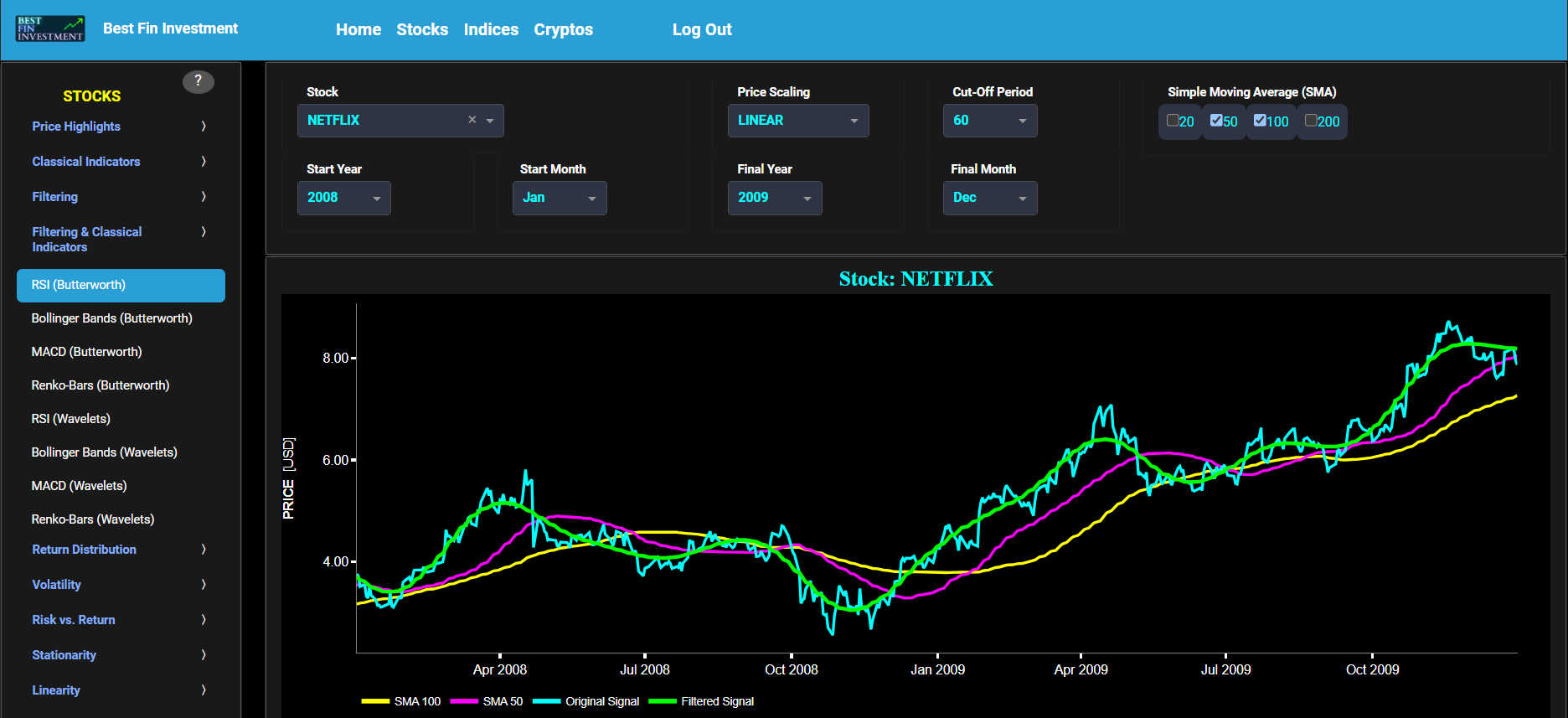
RSI (Butterworth)
This page provides 2 graphs. The upper graph visualizes historical asset prices using daily close prices. In the menu bar (located just above the graphs), you can also select specific time periods to visualize and also toggle between a linear or logarithmic price scaling on the y-axis. In addition the upper graph allows you to superimpose several Simple Moving Average (SMA) lines. Next this page allows you to add a filtered price signal obtained through the application of a causal low-pass Butterworth digital filter. The filter cut-off time period (Tc), with Tc expressed in Days, can also be selected in the menu bar. The purpose of this filter is to smoothen-out the original price signal, i.e. by filtering out (or removing) any high-frequency content (with frequency > 1/Tc), or equivalently, by removing the low-periodic signal content (with period < Tc). Refer also to the lower graph on page "Frequency Analysis" to help you select an appropriate cut-off time period value.
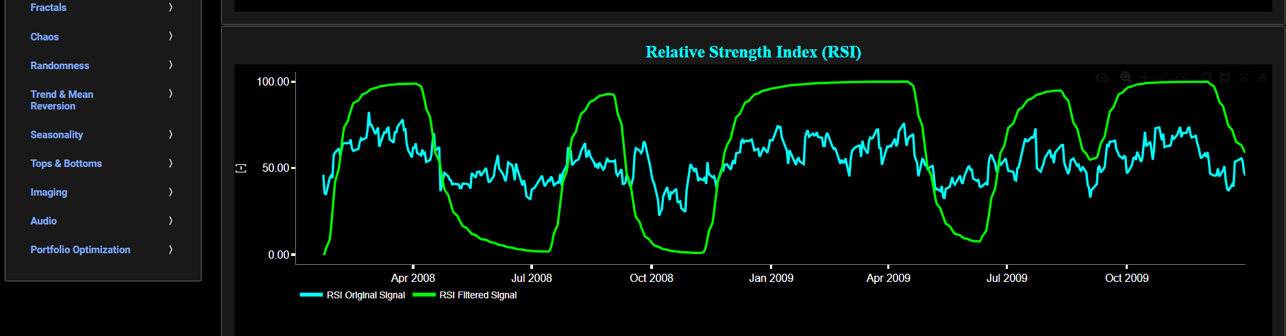
The lower graph presents the standard 14-period Relative Strength Index (RSI) indicator applied to the original (unfiltered) price signal data and subsequently applied to the filtered (Butterworth) price signal data. Finally you can also compare the results obtained on this page with the ones obtained using a Wavelet filter on page “RSI (Wavelets)”.
Filtering & Classical Indicators
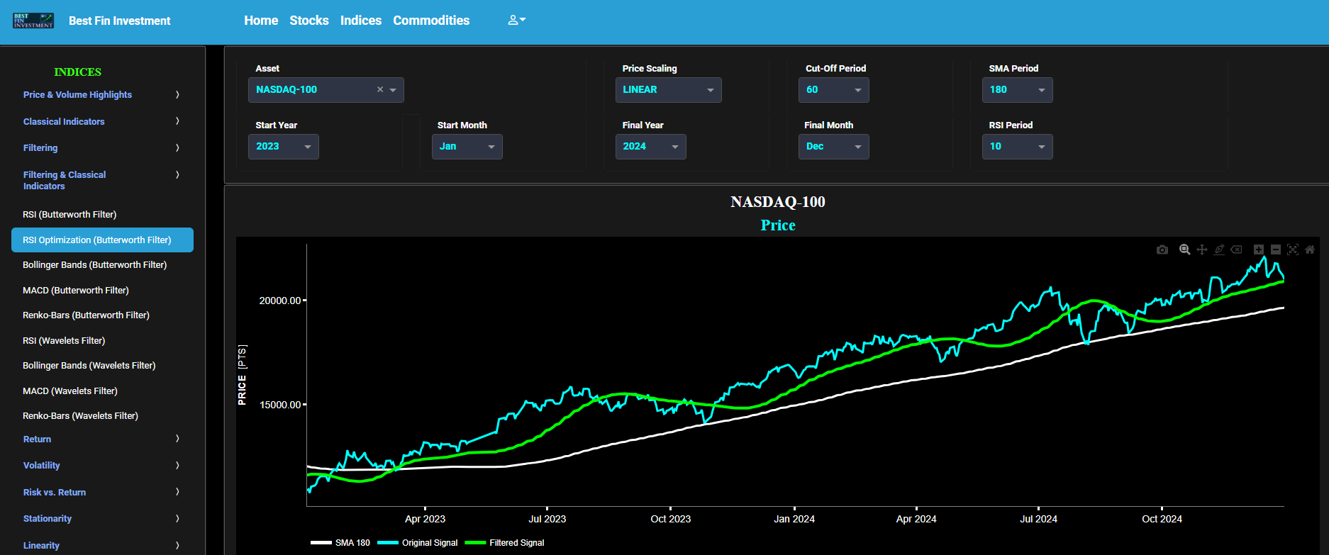
RRSI Optimization (Butterworth Filter)
This page provides 2 graphs. The upper graph visualizes historical asset prices using daily close prices. In the menu bar (located just above the graphs), you can also select specific time periods to visualize and also toggle between a linear or logarithmic price scaling on the y-axis. Next this page allows you to add a filtered price signal obtained through the application of a causal low-pass Butterworth digital filter. The filter cut-off time period (Tc), with Tc expressed in Days, can also be selected in the menu bar. The purpose of this filter is to smoothen-out the original price signal, i.e. by filtering out (or removing) any high-frequency content (with frequency > 1/Tc), or equivalently, by removing the low-periodic signal content (with period < Tc). Refer also to the lower graph on page "Frequency Analysis" to help you select an appropriate cut-off time period value. In addition, the upper graph allows you to superimpose a user-defined Simple Moving Average (SMA) line where its lookback time period (in Days) is set in a dedicated dropdown menu named "SMA Period". This SMA is applied to the original unfiltered price signal.
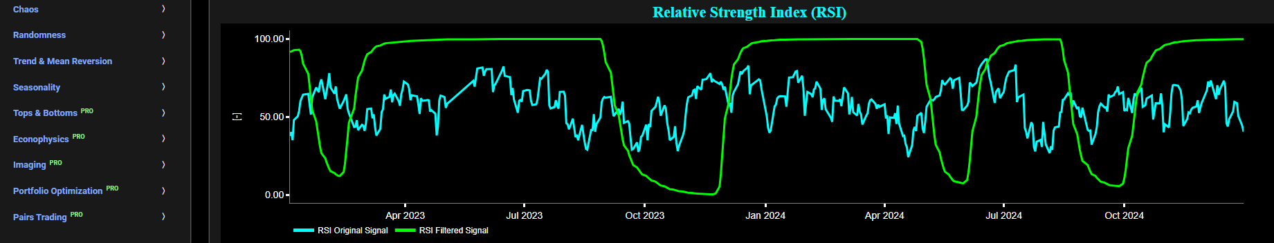
Further, the lower graph also allows you to superimpose a user-defined Relative Strength Index (RSI) line where its lookback time period (in Days) is also set by a dedicated dropdown menu named "RSI Period". This enables you to compare the RSI indicator applied to the original (unfiltered) price signal data with the RSI indicator applied to the filtered (Butterworth) price signal data.
Filtering & Classical Indicators
Bollinger Bands (Butterworth)
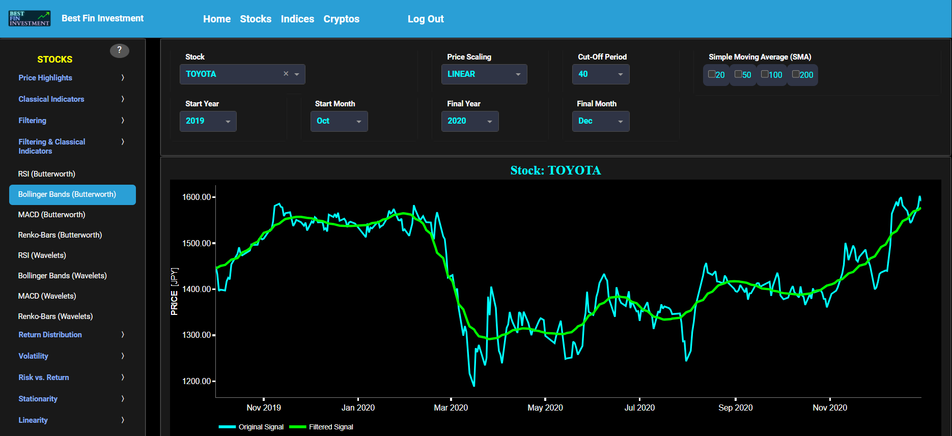
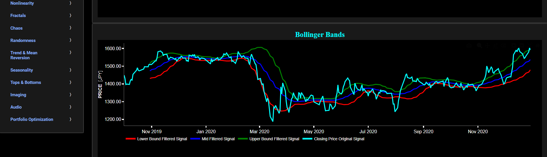
This page provides 2 graphs. The upper graph visualizes historical asset prices using daily close prices. In the menu bar (located just above the graphs), you can also select specific time periods to visualize and also toggle between a linear or logarithmic price scaling on the y-axis. In addition the upper graph allows you to superimpose several Simple Moving Average (SMA) lines. Next this page allows you to add a filtered price signal obtained through the application of a causal low-pass Butterworth digital filter. The filter cut-off time period (Tc), with Tc expressed in Days, can also be selected in the menu bar. The purpose of this filter is to smoothen-out the original price signal, i.e. by filtering out (or removing) any high-frequency content (with frequency > 1/Tc), or equivalently, by removing the low-periodic signal content (with period < Tc). Refer also to the lower graph on page "Frequency Analysis" to help you select an appropriate cut-off time period value.
The lower graph presents the Bollinger Bands indicator (computed on the basis of a standard 20-period moving average) and applied towards the filtered (Butterworth) price signal data. The lower graph also shows, in cyan color, the original (unfiltered) price signal data. Finally you can also compare the results obtained on this page with the ones obtained using a Wavelet filter on page “Bollinger Bands (Wavelets)”.
Filtering & Classical Indicators
MACD (Butterworth)
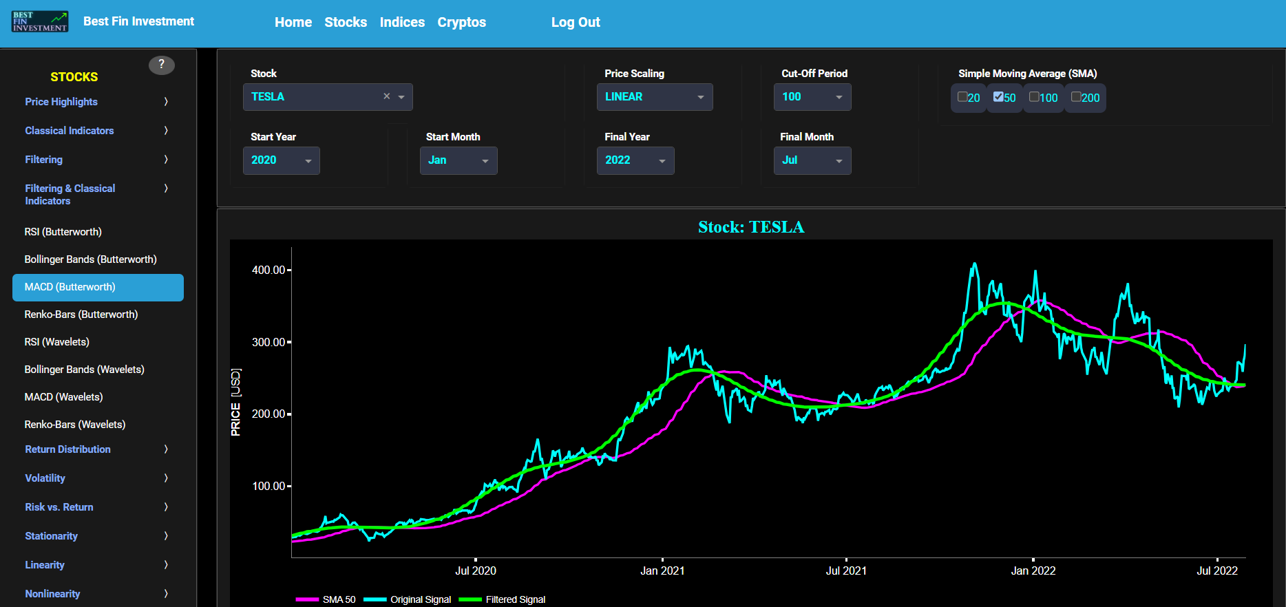
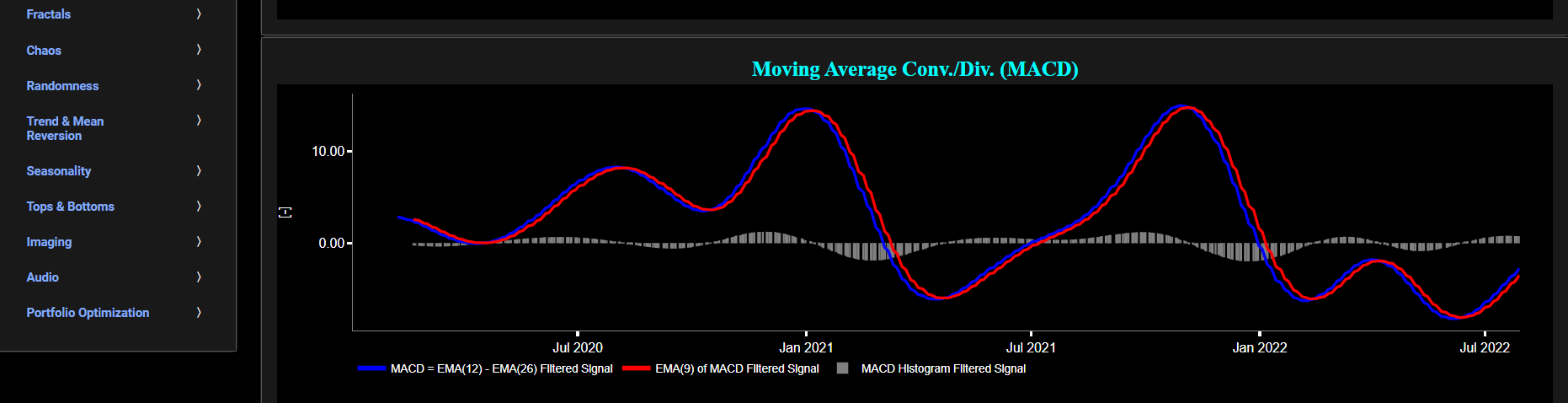
This page provides 2 graphs. The upper graph visualizes historical asset prices using daily close prices. In the menu bar (located just above the graphs), you can also select specific time periods to visualize and also toggle between a linear or logarithmic price scaling on the y-axis. In addition the upper graph allows you to superimpose several Simple Moving Average (SMA) lines. Next this page allows you to add a filtered price signal obtained through the application of a causal low-pass Butterworth digital filter. The filter cut-off time period (Tc), with Tc expressed in Days, can also be selected in the menu bar. The purpose of this filter is to smoothen-out the original price signal, i.e. by filtering out (or removing) any high-frequency content (with frequency > 1/Tc), or equivalently, by removing the low-periodic signal content (with period < Tc). Refer also to the lower graph on page "Frequency Analysis" to help you select an appropriate cut-off time period value.
The lower graph presents the Moving Average Convergence/Divergence (MACD) indicator (using the standard 12,26,9 moving average periods) and applied towards the filtered (Butterworth) price signal data. Finally you can also compare the results obtained on this page with the ones obtained using a Wavelet filter on page “MACD (Wavelets)”.
Filtering & Classical Indicators
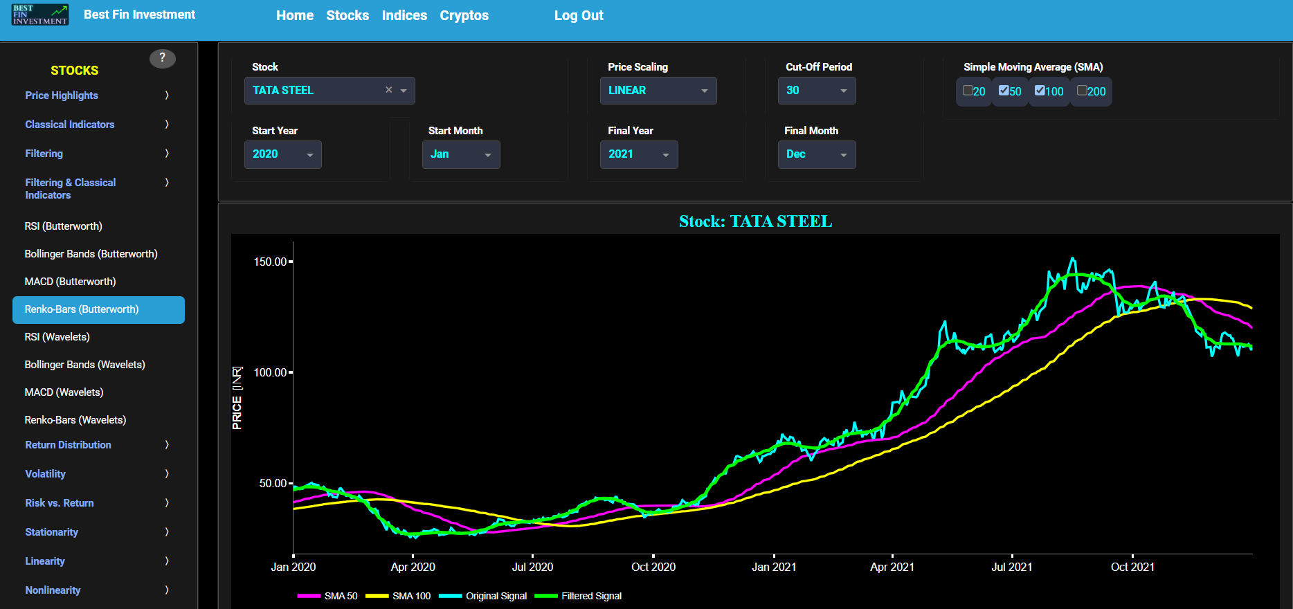
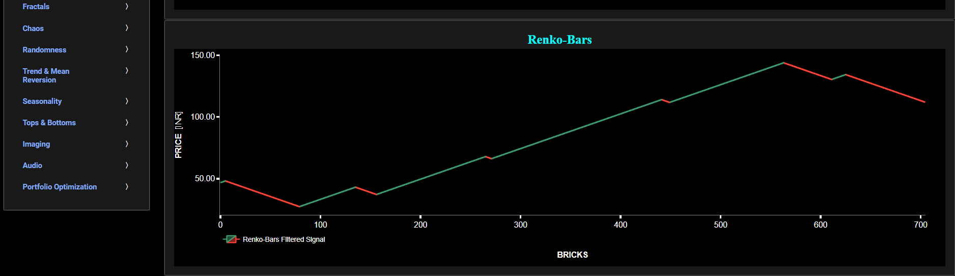
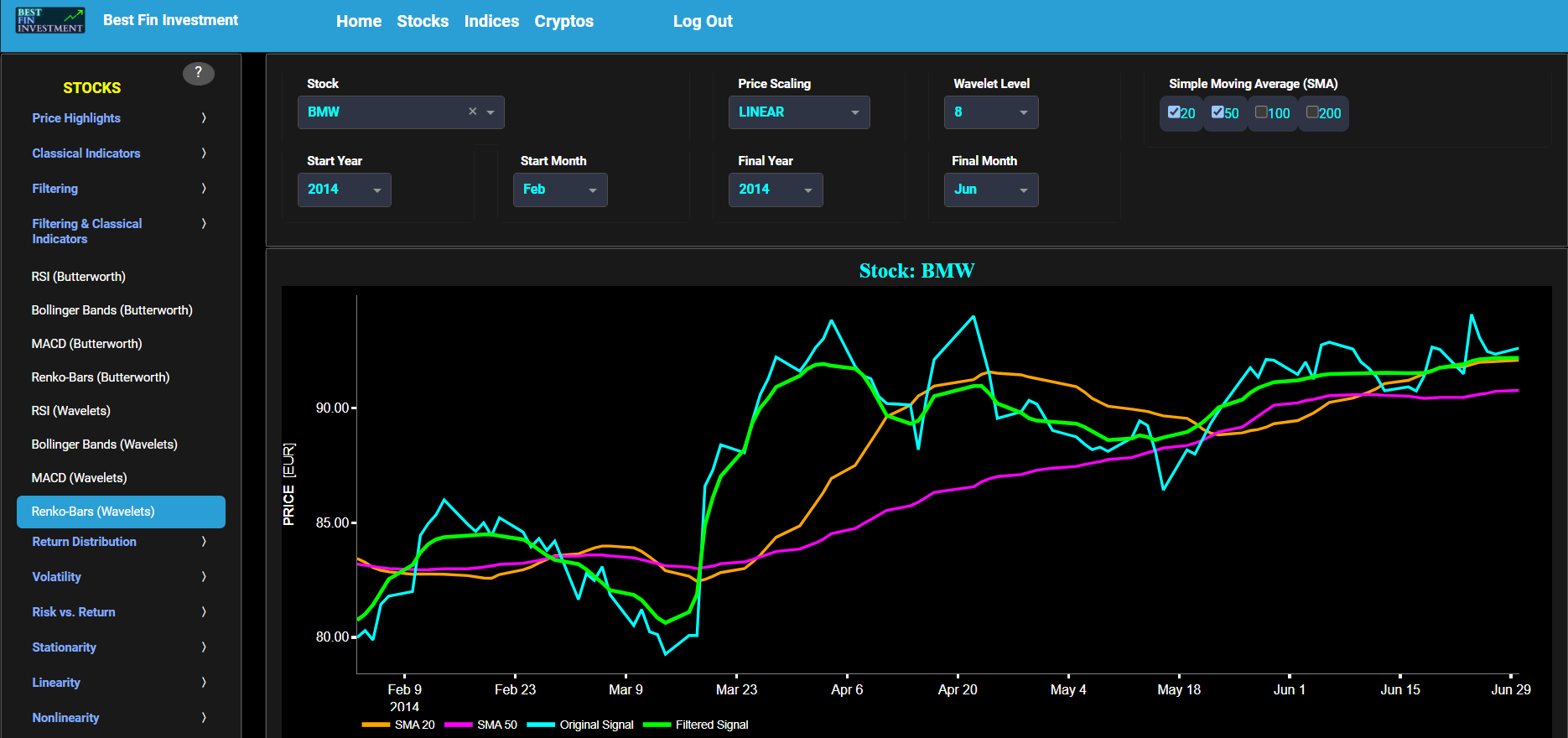
Renko-Bars (Butterworth)
This page provides 2 graphs. The upper graph visualizes historical asset prices using daily close prices. In the menu bar (located just above the graphs), you can also select specific time periods to visualize and also toggle between a linear or logarithmic price scaling on the y-axis. In addition the upper graph allows you to superimpose several Simple Moving Average (SMA) lines. Next this page allows you to add a filtered price signal obtained through the application of a causal low-pass Butterworth digital filter. The filter cut-off time period (Tc), with Tc expressed in Days, can also be selected in the menu bar. The purpose of this filter is to smoothen-out the original price signal, i.e. by filtering out (or removing) any high-frequency content (with frequency > 1/Tc), or equivalently, by removing the low-periodic signal content (with period < Tc). Refer also to the lower graph on page "Frequency Analysis" to help you select an appropriate cut-off time period value.
The lower graph presents the Renko Candle Bars indicator, using a simplified Average True Range (ATR) indicator, and applied towards the filtered (Butterworth) price signal data. Finally you can also compare the results obtained on this page with the ones obtained using a Wavelet filter on page “Renko-Bars (Wavelets)”.
Filtering & Classical Indicators
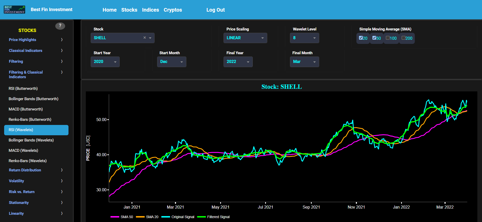
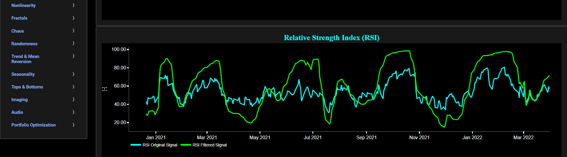
RSI (Wavelets)
This page provides 2 graphs. The upper graph visualizes historical asset prices using daily close prices. In the menu bar (located just above the graphs), you can also select specific time periods to visualize and also toggle between a linear or logarithmic price scaling on the y-axis. In addition the upper graph allows you to superimpose several Simple Moving Average (SMA) lines. Next this page allows you to add a filtered price signal obtained through the application of a Wavelet-based denoising filter. Here we have used the "sym" (symmetric) wavelet family which tends to have good time-frequency localization properties and hence may be better suited for denoising non-stationary financial price data. The so-called Wavelet filter decomposition level can also be selected in the menu bar. The purpose of this filter is to smoothen-out the original price signal, i.e. by filtering out (or removing) any high-frequency content.
The lower graph presents the standard 14-period Relative Strength Index (RSI) indicator applied to the original (unfiltered) price signal data and subsequently applied to the filtered (Wavelets) price signal data. Finally you can also compare the results obtained on this page with the ones obtained using a Butterworth filter on page “RSI (Butterworth)”.
Filtering & Classical Indicators
Bollinger Bands (Wavelets)
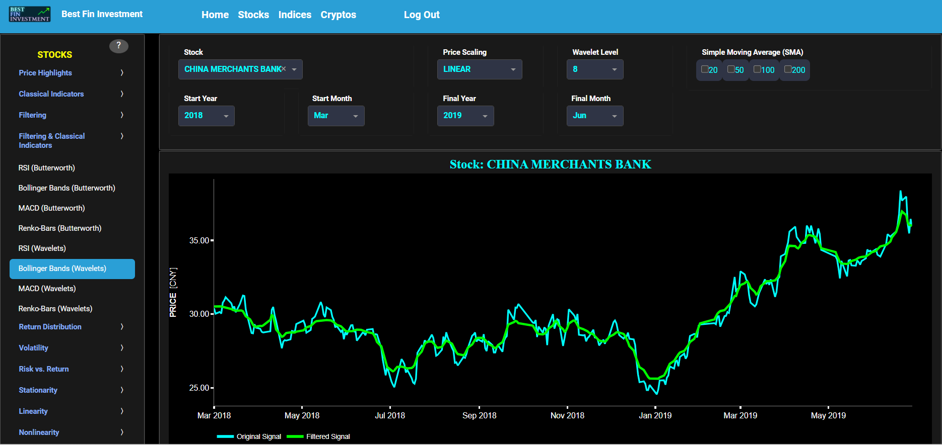
This page provides 2 graphs. The upper graph visualizes historical asset prices using daily close prices. In the menu bar (located just above the graphs), you can also select specific time periods to visualize and also toggle between a linear or logarithmic price scaling on the y-axis. In addition the upper graph allows you to superimpose several Simple Moving Average (SMA) lines. Next this page allows you to add a filtered price signal obtained through the application of a Wavelet-based denoising filter. Here we have used the "sym" (symmetric) wavelet family which tends to have good time-frequency localization properties and hence may be better suited for denoising non-stationary financial price data. The so-called Wavelet filter decomposition level can also be selected in the menu bar. The purpose of this filter is to smoothen-out the original price signal, i.e. by filtering out (or removing) any high-frequency content.
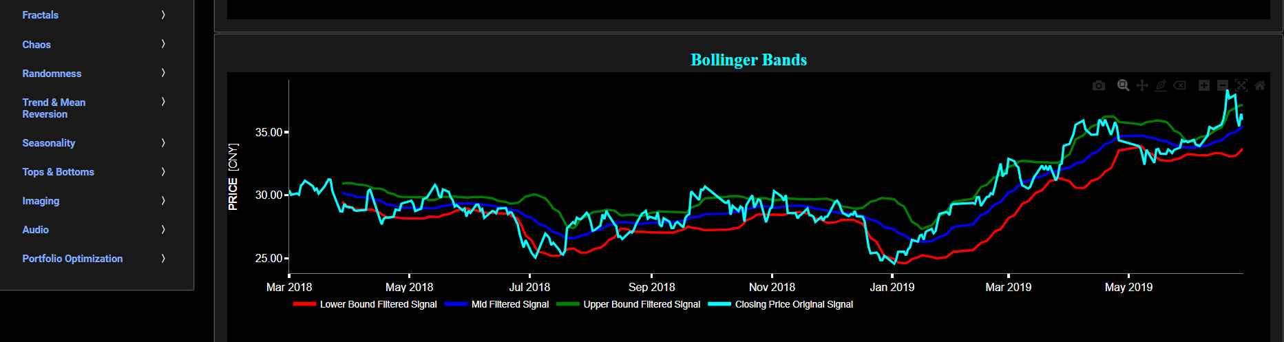
The lower graph presents the Bollinger Bands indicator (computed on the basis of a standard 20-period moving average) and applied towards the filtered (Wavelets) price signal data. The lower graph also shows, in cyan color, the original (unfiltered) price signal data. Finally you can also compare the results obtained on this page with the ones obtained using a Butterworth filter on page “Bollinger Bands (Butterworth)”.
Filtering & Classical Indicators
MACD (Wavelets)
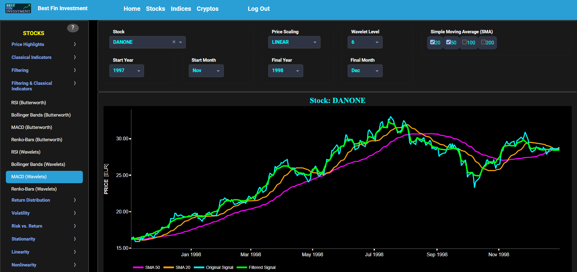
This page provides 2 graphs. The upper graph visualizes historical asset prices using daily close prices. In the menu bar (located just above the graphs), you can also select specific time periods to visualize and also toggle between a linear or logarithmic price scaling on the y-axis. In addition the upper graph allows you to superimpose several Simple Moving Average (SMA) lines. Next this page allows you to add a filtered price signal obtained through the application of a Wavelet-based denoising filter. Here we have used the "sym" (symmetric) wavelet family which tends to have good time-frequency localization properties and hence may be better suited for denoising non-stationary financial price data. The so-called Wavelet filter decomposition level can also be selected in the menu bar. The purpose of this filter is to smoothen-out the original price signal, i.e. by filtering out (or removing) any high-frequency content.
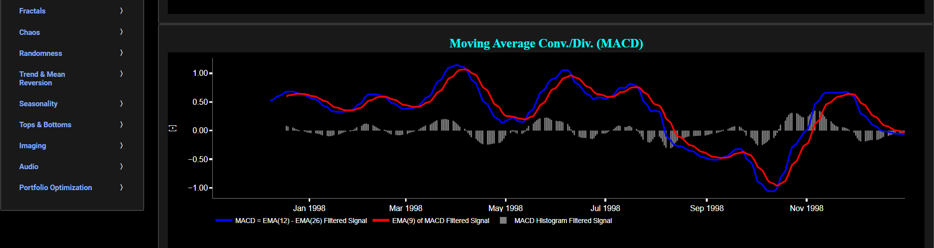
The lower graph presents the Moving Average Convergence/Divergence (MACD) indicator (using the standard 12,26,9 moving average periods) and applied towards the filtered (Wavelets) price signal data. Finally you can also compare the results obtained on this page with the ones obtained using a Butterworth filter on page “MACD (Butterworth)”.
Filtering & Classical Indicators
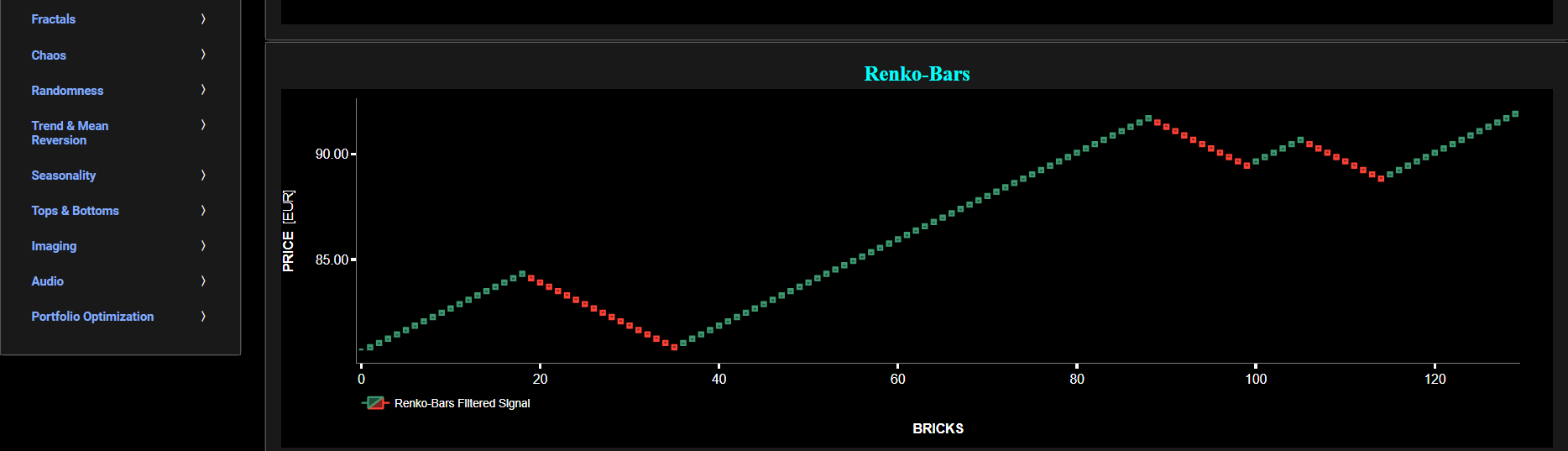
Renko-Bars (Wavelets)
This page provides 2 graphs. The upper graph visualizes historical asset prices using daily close prices. In the menu bar (located just above the graphs), you can also select specific time periods to visualize and also toggle between a linear or logarithmic price scaling on the y-axis. In addition the upper graph allows you to superimpose several Simple Moving Average (SMA) lines. Next this page allows you to add a filtered price signal obtained through the application of a Wavelet-based denoising filter. Here we have used the "sym" (symmetric) wavelet family which tends to have good time-frequency localization properties and hence may be better suited for denoising non-stationary financial price data. The so-called Wavelet filter decomposition level can also be selected in the menu bar. The purpose of this filter is to smoothen-out the original price signal, i.e. by filtering out (or removing) any high-frequency content.
The lower graph presents the Renko Candle Bars indicator, using a simplified Average True Range (ATR) indicator, and applied towards the filtered (Wavelets) price signal data. Finally you can also compare the results obtained on this page with the ones obtained using a Butterworth filter on page “Renko-Bars (Butterworth)”.
Return
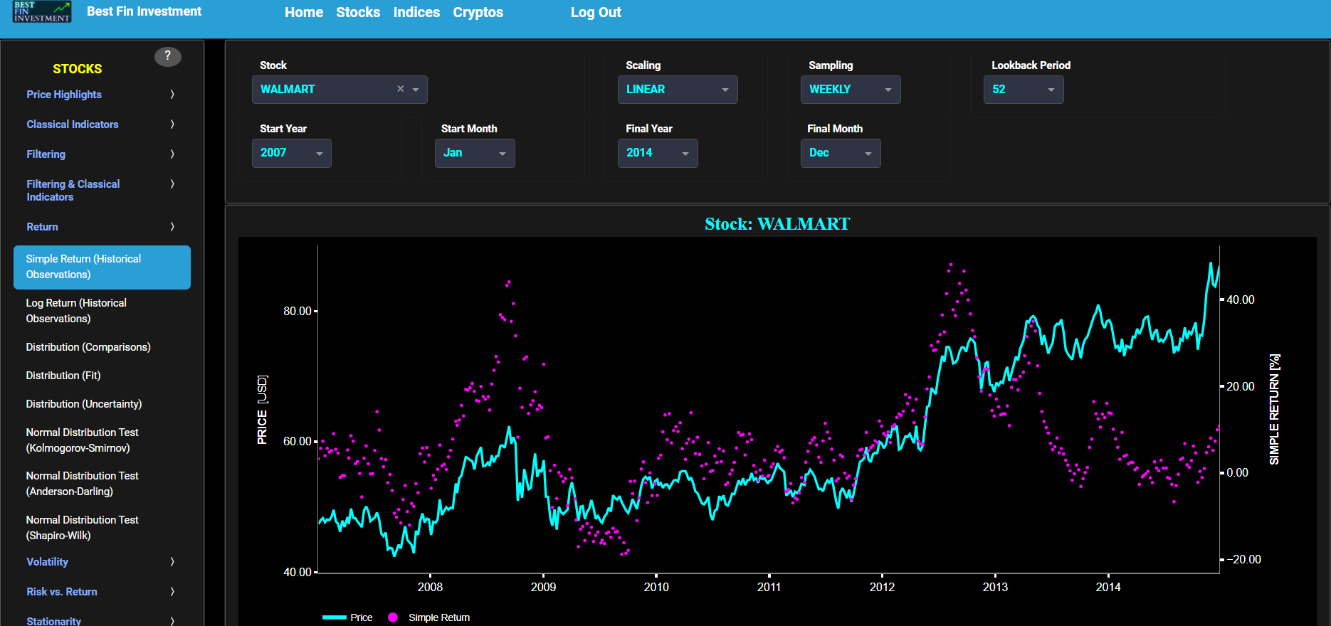
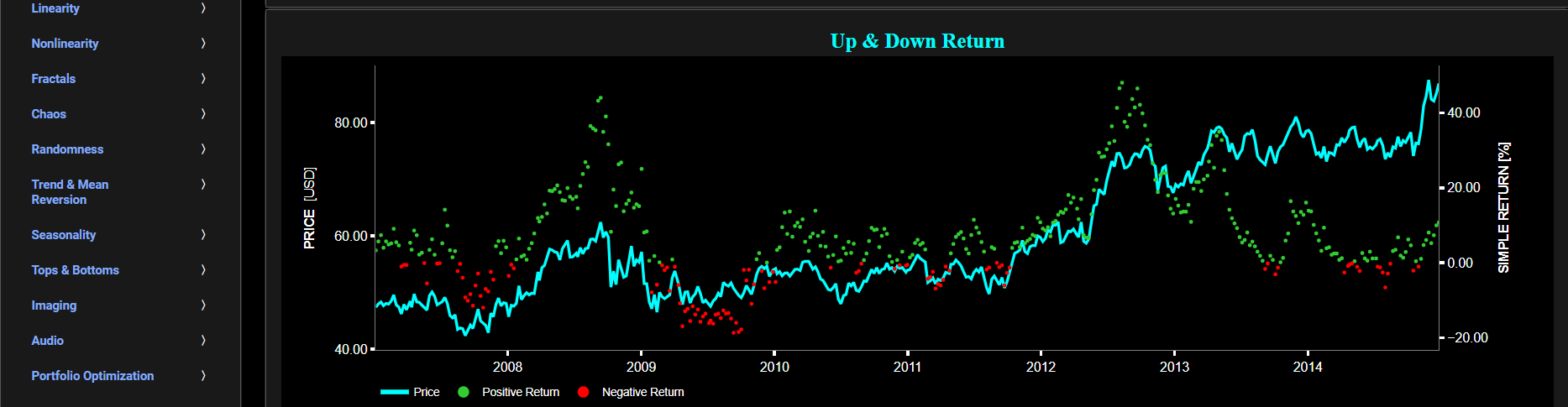
Simple Return (Historical Observations)
This page provides 2 graphs. The upper graph visualizes historical asset prices in cyan color using either daily, weekly, or monthly close prices. In the menu bar (located just above the graphs), you can also select specific time periods to visualize and also toggle between a linear or logarithmic price scaling on the left y-axis. Next to the cyan line, the upper graph also visualizes the historical asset return. Here, return is defined as the simple asset return which is quantified as the percentage change in the asset's price between consecutive time periods. This return is shown in magenta and expressed on the right y-axis. The return is computed using a lookback time period that is selected in the menu bar (located just above the graphs). The lower graph is somewhat similar to the upper graph except that it shows the positive price returns in green and negative price returns in red.
Return
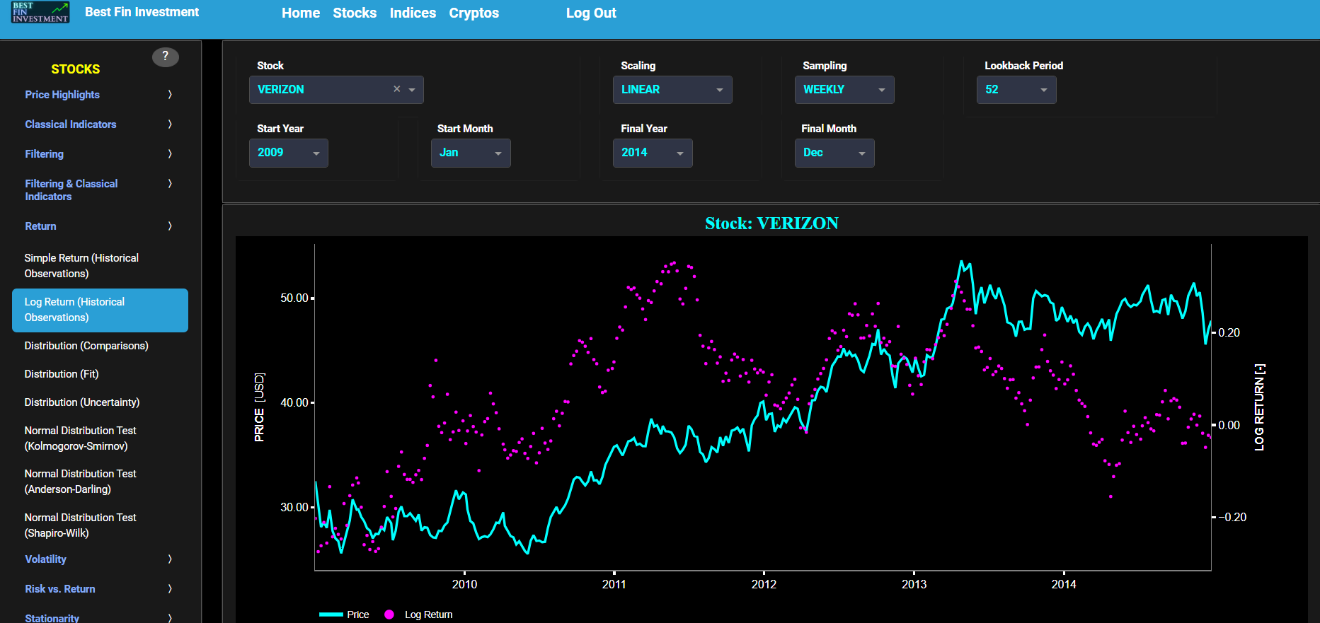
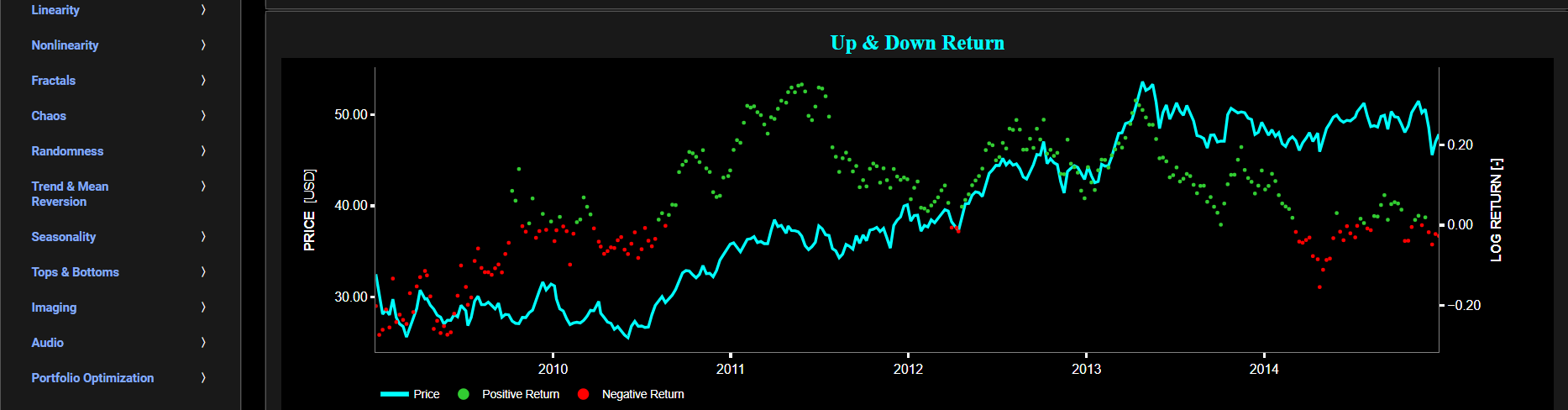
Log Return (Historical Observations)
This page provides 2 graphs. The upper graph visualizes historical asset prices in cyan color using either daily, weekly, or monthly close prices. In the menu bar (located just above the graphs), you can also select specific time periods to visualize and also toggle between a linear or logarithmic price scaling on the left y-axis. Next to the cyan line, the upper graph also visualizes the historical asset log return. Here, log return is defined as the natural logarithm of the asset price percentage change between consecutive time periods. This return is shown in magenta and expressed on the right y-axis. The return is computed using a lookback time period that is selected in the menu bar (located just above the graphs). The lower graph is somewhat similar to the upper graph except that it shows the positive price returns in green and negative price returns in red.
Return
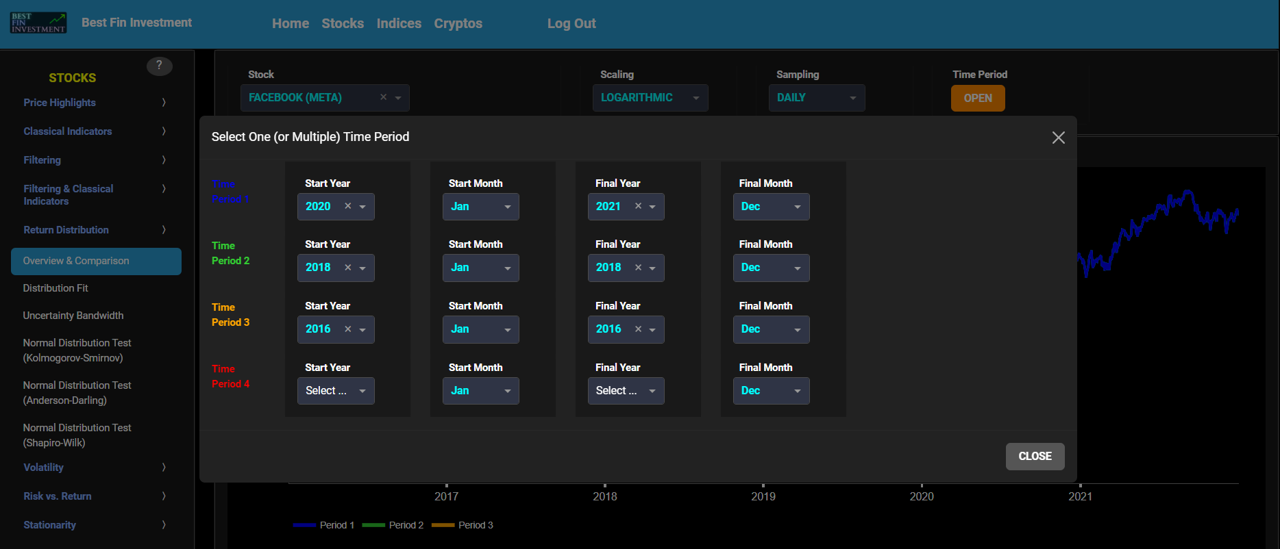
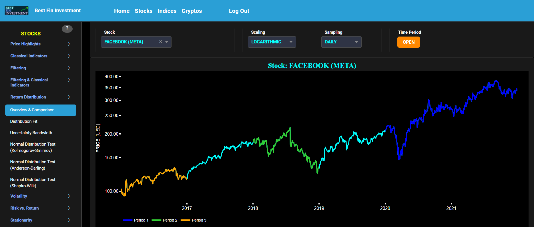
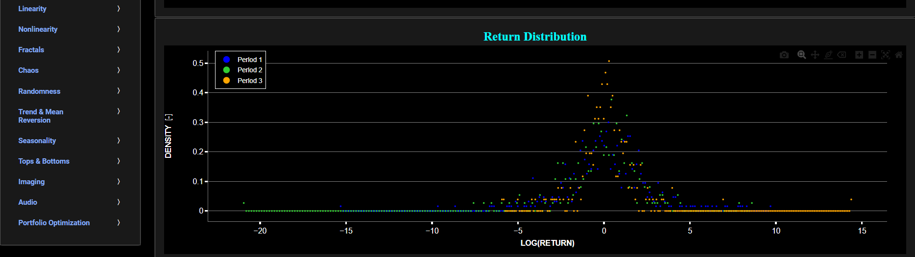
Distribution (Comparisons)
This page provides 2 graphs. The upper graph visualizes historical asset prices using either daily, weekly, or monthly close prices. In the menu bar (located just above the graphs), you can also toggle between a linear or logarithmic price scaling on the y-axis. Further you can select up to 4 specific time periods for comparisons of return distributions. Here price “return” is defined as the % change between 2 consecutive close prices. The lower graph visualizes the corresponding return distributions for the selected asset price data. Note that if logarithmic scaling is selected, the lower graph will then provide the distribution of the logarithm of price returns.
Return
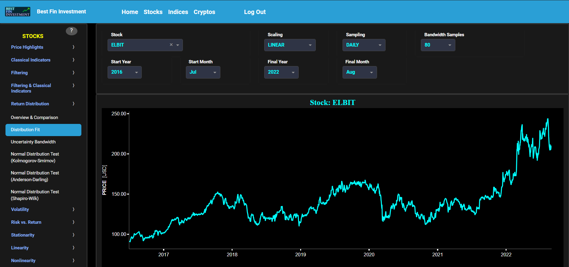
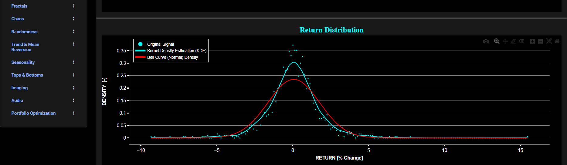
Distribution (Fit)
This page provides 2 graphs. The upper graph visualizes historical asset prices using either daily, weekly, or monthly close prices. In the menu bar (located just above the graphs), you can also select specific time periods to visualize and also toggle between a linear or logarithmic price scaling on the y-axis. The lower graph visualizes the corresponding return distributions for the selected asset price data. Note that if logarithmic scaling is selected, the lower graph will then provide the distribution of the logarithm of price returns. Further, the lower graph also presents 2 additional lines. The line shown in red represents a normal density fit of the price return data, whereas the second line shown in cyan represents a fit from a Kernel Density Estimator (KDE) using “exponential” type kernels. In the menu bar (located just above the graphs), you can also select the number of bandwidth samples that will be used during the KDE identification process. The higher the number of bandwidth samples, the better the density fit albeit at the expense of increased computational cost. Once the number of bandwidth samples is selected the algorithm will then search for the optimal KDE bandwidth using a so-called leave-one-out cross-validation procedure.
Return
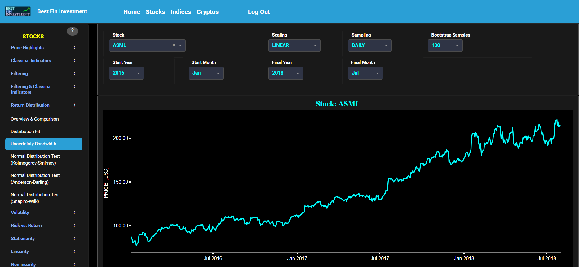
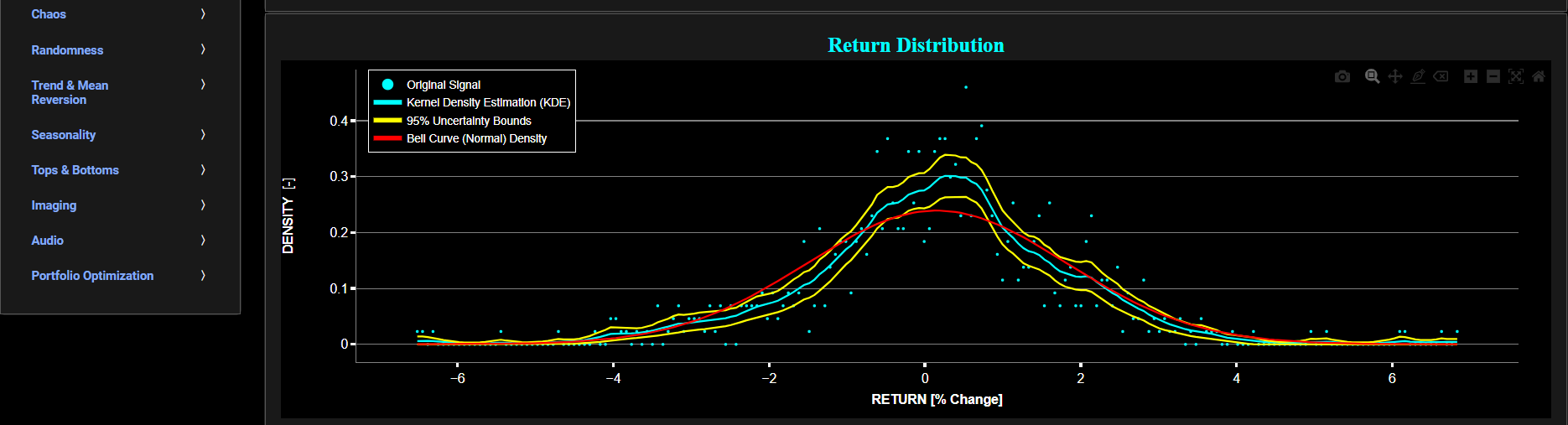
Distribution (Uncertainty)
This page provides 2 graphs. The upper graph visualizes historical asset prices using either daily, weekly, or monthly close prices. In the menu bar (located just above the graphs), you can also select specific time periods to visualize and also toggle between a linear or logarithmic price scaling on the y-axis. The lower graph visualizes the corresponding return distributions for the selected asset price data. Note that if logarithmic scaling is selected, the lower graph will then provide the distribution of the logarithm of price returns. Further, the lower graph also presents 4 additional lines. The line shown in red represents a normal density fit of the price return data, whereas the line shown in cyan represents a fit from a Kernel Density Estimator (KDE) using “exponential” type kernels. The 2 yellow lines represent the 95% confidence interval (or uncertainty bounds) around the cyan line, obtained through a bootstrapping procedure. In the menu bar (located just above the graphs), you can also select the number of bootstrap samples that will be used during the confidence interval estimation. This number is also used during the KDE identification process. Note that the higher the number of bootstrap samples, the better the confidence interval estimation albeit at the expense of increased computational cost.
Return
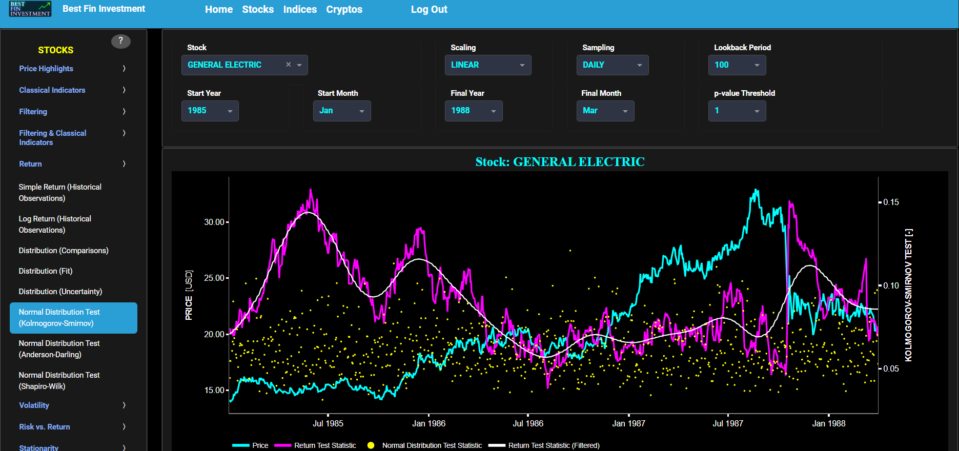
Normal Distribution Test (Kolmogorov-Smirnov)
This page provides 2 graphs. The upper graph visualizes historical asset prices in cyan color using either daily, weekly, or monthly close prices. In the menu bar (located just above the graphs), you can also select specific time periods to visualize and also toggle between a linear or logarithmic price scaling on the y-axis. Next to the cyan line, the upper graph also visualizes the test statistic for the one-sample Kolmogorov-Smirnov (KS) normal distribution test for the asset incremental returns (i.e. % change) in magenta, and for synthetically generated normally distributed independent and identically distributed (i.i.d.) returns in yellow. The yellow data points are given here for reference and comparison purposes (i.e. benchmarking). Next the white line represents a filtered version of the magenta line through the application of a low-pass Butterworth digital filter. The one-sample KS test compares the underlying distribution (the sample returns of the selected asset) against a given normal (i.e. Gaussian) distribution. The null hypothesis consists in having the sample returns distributed according to the standard normal distribution. The KS test statistic represents a measure of how well the sample data matches the theoretical normal distribution. A larger KS statistic indicates a greater discrepancy from normal distribution.
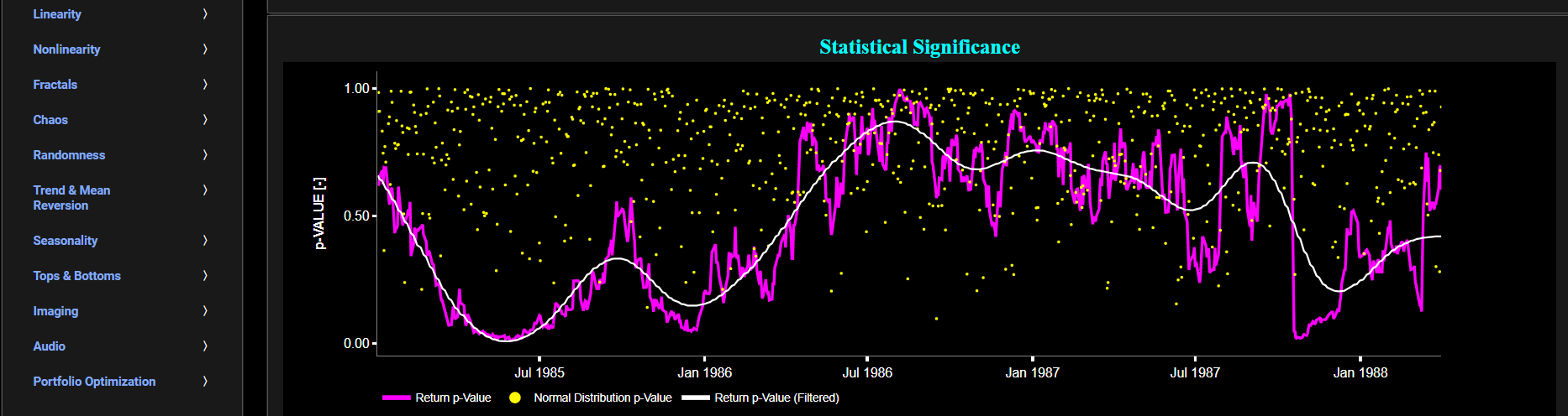
Next the lower graph visualizes the statistical significance (or so called p-value) for the KS test and for the benchmark signal. It is often typical to choose a confidence level of 95%; meaning that we will reject the null hypothesis in favor of the alternative (i.e. the data does not follow a standard normal distribution) if the test statistic p-value is less than 0.05. Finally in the menu bar (located just above the graphs), you can also select specific values for the lookback time period on which the KS test will be computed as well as set a maximum p-value visualization threshold pM, i.e. by only showing the data points for which we have p-value < pM.
Return
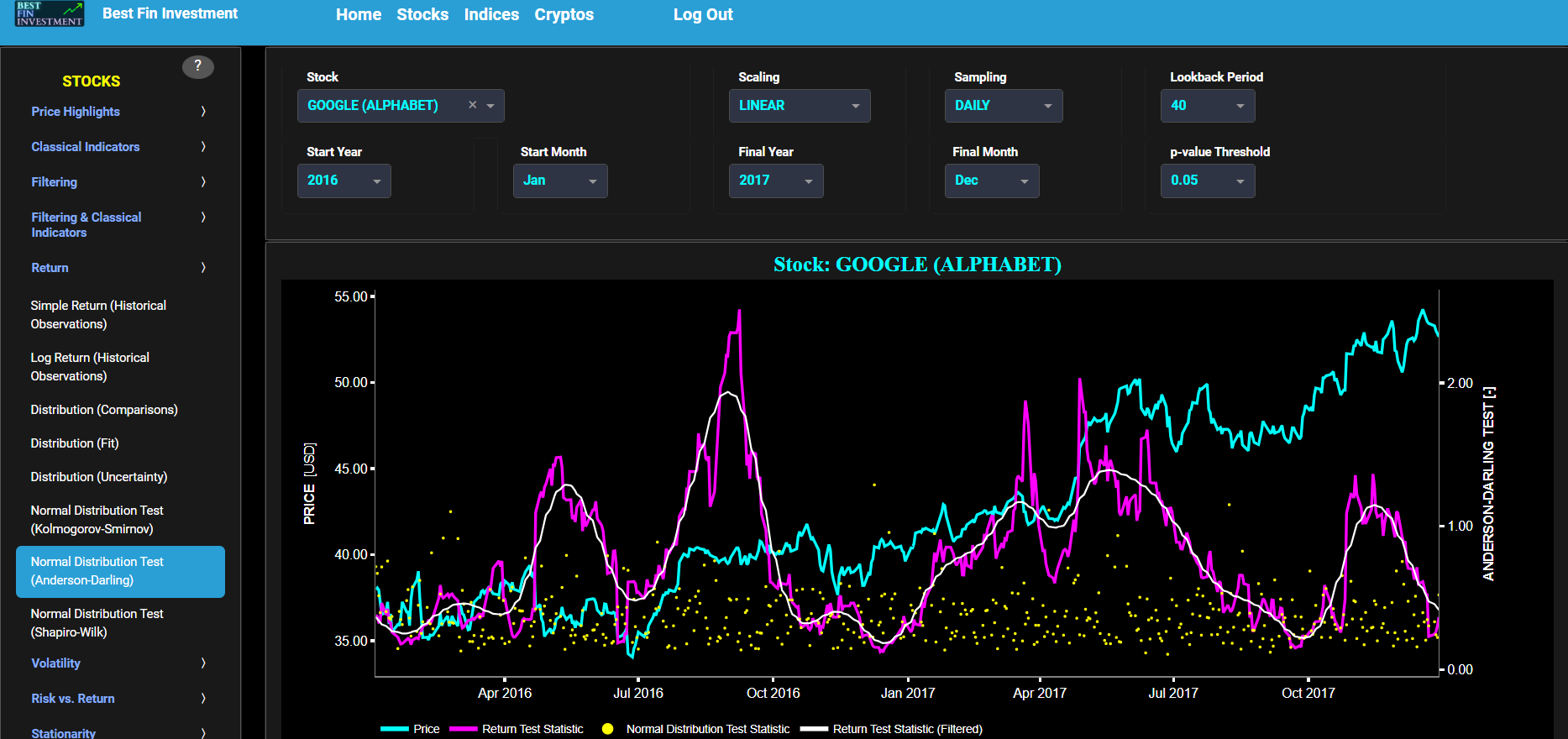
Normal Distribution Test (Anderson-Darling)
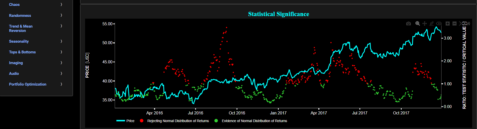
This page provides 2 graphs. The upper graph visualizes historical asset prices in cyan color using either daily, weekly, or monthly close prices. In the menu bar (located just above the graphs), you can also select specific time periods to visualize and also toggle between a linear or logarithmic price scaling on the y-axis. Next to the cyan line, the upper graph also visualizes the test statistic for the Anderson-Darling (AD) normal distribution test for the asset incremental returns (i.e. % change) in magenta, and for synthetically generated normally distributed independent and identically distributed (i.i.d.) returns in yellow. The yellow data points are given here for reference and comparison purposes (i.e. benchmarking). Next the white line represents a filtered version of the magenta line through the application of a low-pass Butterworth digital filter. The AD test compares the underlying distribution (the sample returns of the selected asset) against a given normal (i.e. Gaussian) distribution. The null hypothesis consists in having the sample returns distributed according to the standard normal distribution. The AD test statistic represents a measure of how well the sample data matches the theoretical normal distribution. A larger AD statistic indicates a greater discrepancy from normal distribution.
Next the lower graph visualizes the ratio of test statistic divided by test critical value at a selected p-value threshold. The p-value corresponds to the statistical significance of the AD test. In other words, if the returned statistic is larger than the critical value (i.e. ratio > 1) then for the corresponding chosen p-value significance level, the null hypothesis that the data comes from a normal distribution can be rejected. Note that it is often typical to choose a confidence level of 95% (i.e. p-value less than 0.05). Finally in the menu bar (located just above the graphs), you can also select specific values for the lookback time period on which the AD test will be computed as well as set a maximum p-value visualization threshold pM, i.e. by only showing the data points for which we have p-value < pM.
Return
Normal Distribution Test (Shapiro-Wilk)
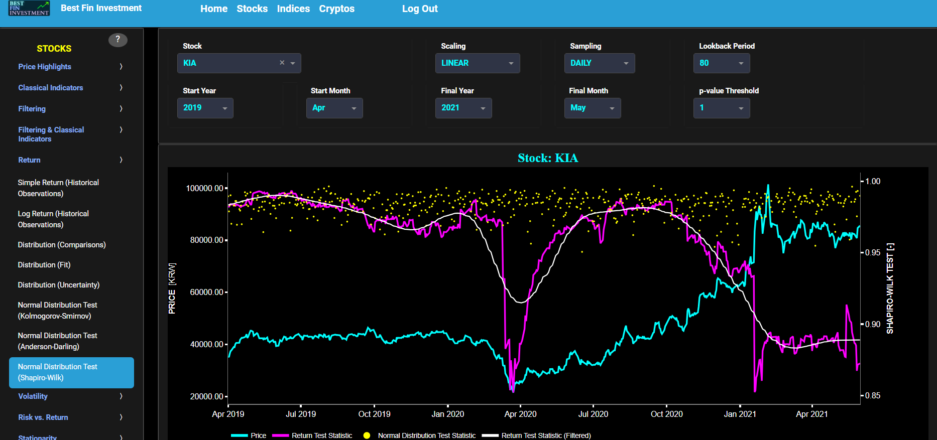
This page provides 2 graphs. The upper graph visualizes historical asset prices in cyan color using either daily, weekly, or monthly close prices. In the menu bar (located just above the graphs), you can also select specific time periods to visualize and also toggle between a linear or logarithmic price scaling on the y-axis. Next to the cyan line, the upper graph also visualizes the test statistic for the Shapiro-Wilk (SW) normal distribution test for the asset incremental returns (i.e. % change) in magenta, and for synthetically generated normally distributed independent and identically distributed (i.i.d.) returns in yellow. The yellow data points are given here for reference and comparison purposes (i.e. benchmarking). Next the white line represents a filtered version of the magenta line through the application of a low-pass Butterworth digital filter. The SW test compares the underlying distribution (the sample returns of the selected asset) against a given normal (i.e. Gaussian) distribution. The null hypothesis consists in having the sample returns distributed according to the standard normal distribution. The SW test statistic measures the degree of departure from a normal distribution. It is based on the covariances between the ordered data values and the expected values under the assumption of normality. The test statistic tends to be close to 1 for normally distributed data and smaller for data that deviate from normality.
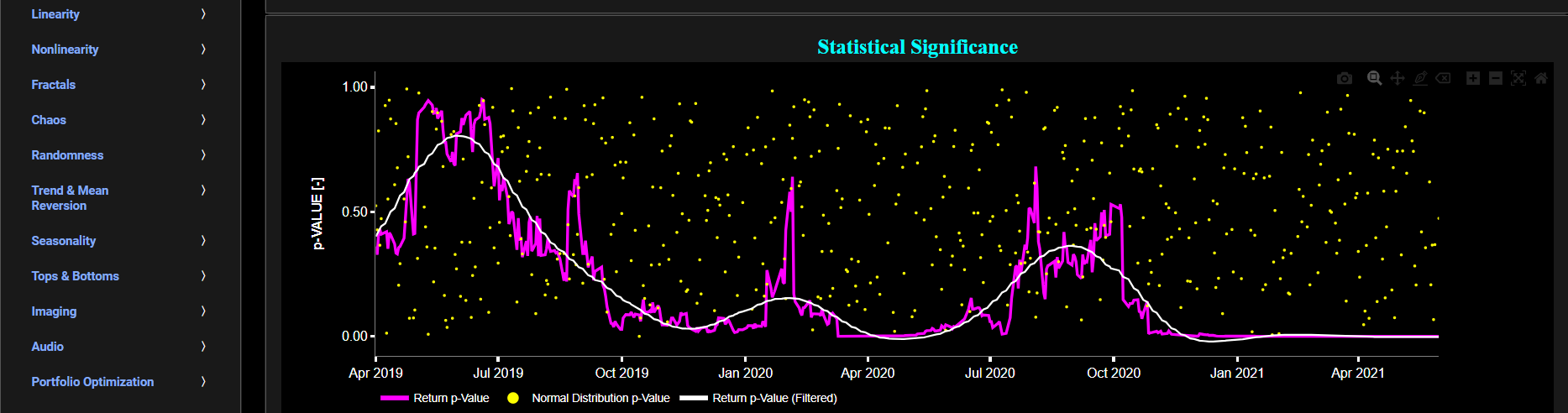
Next the lower graph visualizes the statistical significance (or so called p-value) for the SW test and for the benchmark signal. It is often typical to choose a confidence level of 95%; meaning that we will reject the null hypothesis in favor of the alternative (i.e. the data does not follow a standard normal distribution) if the test statistic p-value is less than 0.05. Finally in the menu bar (located just above the graphs), you can also select specific values for the lookback time period on which the SW test will be computed as well as set a maximum p-value visualization threshold pM, i.e. by only showing the data points for which we have p-value < pM.
Volatility
Historical Observations
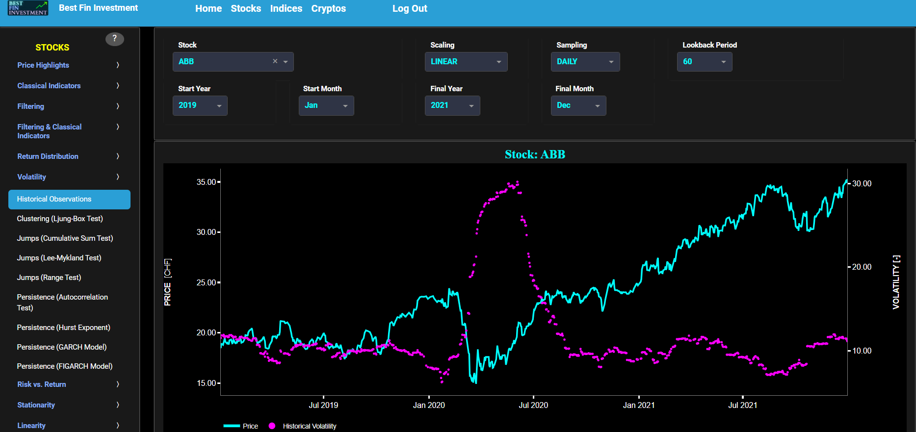
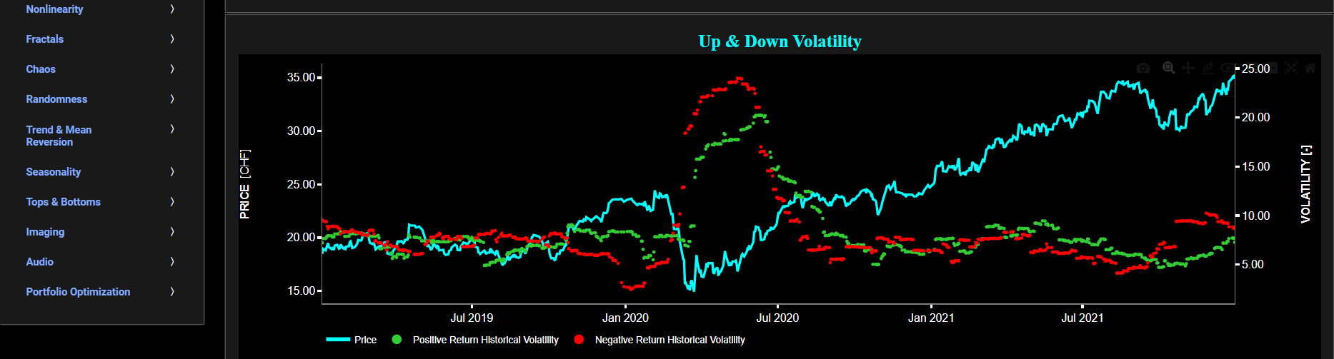
This page provides 2 graphs. The upper graph visualizes historical asset prices in cyan color using either daily, weekly, or monthly close prices. In the menu bar (located just above the graphs), you can also select specific time periods to visualize and also toggle between a linear or logarithmic price scaling on the left y-axis. Next to the cyan line, the upper graph also visualizes the historical asset volatility. This volatility is shown in magenta and expressed on the right y-axis. The volatility is computed using a lookback time period that is selected in the menu bar (located just above the graphs). The lower graph is somewhat similar to the upper graph except that it shows the historical volatility of positive price returns in green and historical volatility of negative price returns in red.
Volatility
Clustering (Ljung-Box Test)
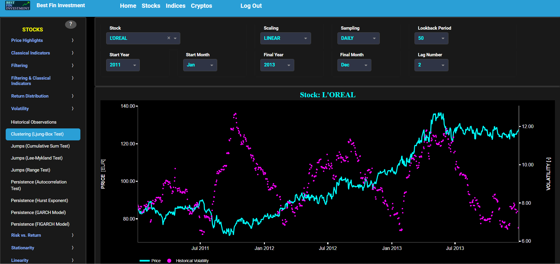
This page provides 3 graphs. The upper graph visualizes historical asset prices in cyan color using either daily, weekly, or monthly close prices. In the menu bar (located just above the graphs), you can also select specific time periods to visualize and also toggle between a linear or logarithmic price scaling on the left y-axis. Next to the cyan line, the upper graph also visualizes the historical asset volatility. This volatility is shown in magenta and expressed on the right y-axis. The volatility is computed using a lookback time period that is selected in the menu bar (located just above the graphs).
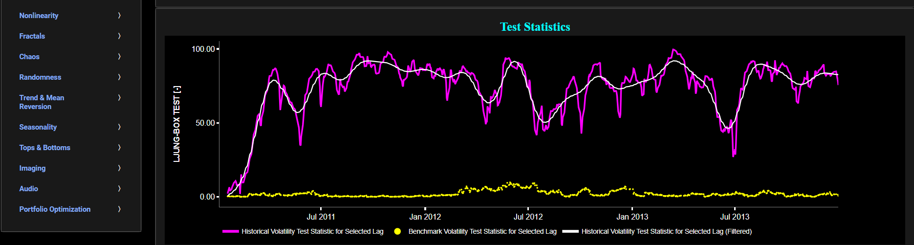
The middle graph visualizes the statistic for the Ljung-Box autocorrelation (LB) test for the asset volatility in magenta, and for a benchmark time series in yellow. This benchmark signal is based upon synthetically generated, normally distributed, independent and identically distributed (i.i.d.) returns. For this benchmark signal, each step is independent of the previous steps, and there is no systematic trend or pattern in the data. The yellow data points are given here for reference and comparison purposes (hence benchmarking). Next the white line represents a filtered version of the magenta line through the application of a low-pass Butterworth digital filter. Now the LB test is a statistical test used to check for the presence of autocorrelation in a time series. In the context of financial time series, autocorrelation can be indicative of volatility clustering. The null hypothesis of the LB test assumes that there is no autocorrelation in the time series data. In other words, it assumes that the data points are independently and identically distributed (i.i.d.), which would imply no clustering of volatility. The alternative hypothesis suggests the presence of autocorrelation in the time series data, indicating volatility clustering. Now a high LB test value would suggest that there is autocorrelation in the time series data. This implies that there are periods of high volatility followed by periods of low volatility, indicating volatility clustering. Further, you can test this autocorrelation for specific time series lags, with the latter being selected in the menu bar (located just above the graphs).
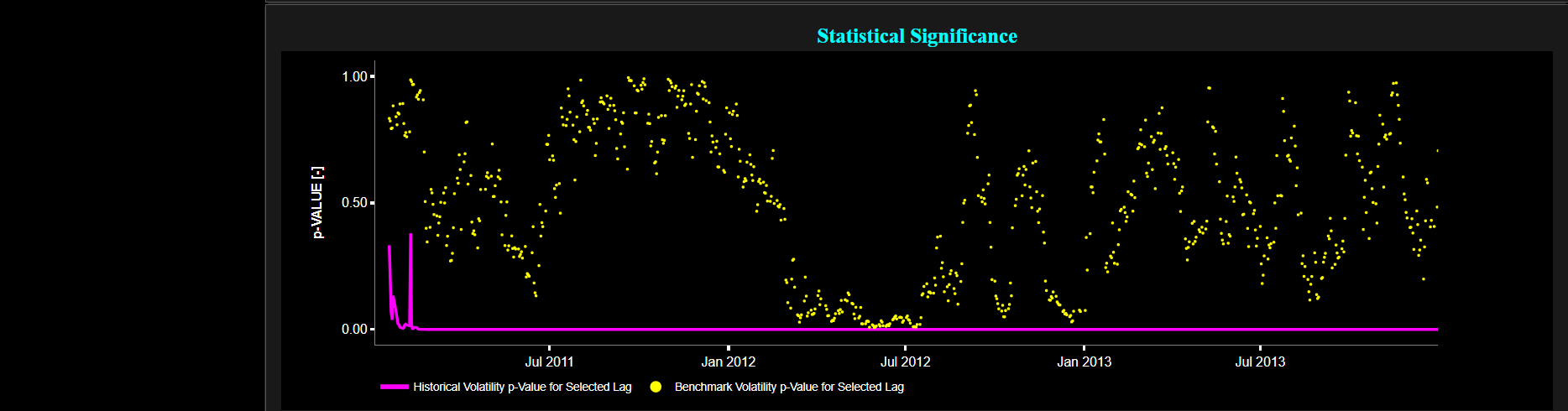
Finally the lower graph visualizes the statistical significance of the LB autocorrelation test for the asset volatility in magenta, and for the benchmark signal in yellow. It is often typical to choose a confidence level of 95%; meaning that we will reject the null hypothesis in favor of the alternative (i.e. meaning that there is significant autocorrelation in the data, which implies the presence of volatility clustering) if the test statistic p-value is less than 0.05.
Volatility
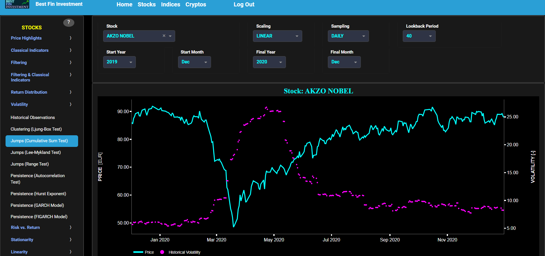
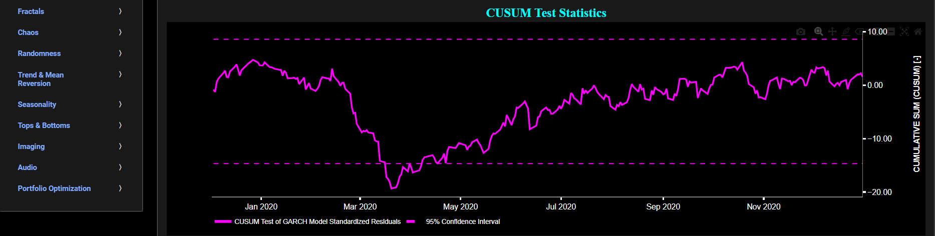
Jumps (Cumulative Sum Test)
This page provides 2 graphs. The upper graph visualizes historical asset prices in cyan color using either daily, weekly, or monthly close prices. In the menu bar (located just above the graphs), you can also select specific time periods to visualize and also toggle between a linear or logarithmic price scaling on the left y-axis. Next to the cyan line, the upper graph also visualizes the historical asset volatility. This volatility is shown in magenta and expressed on the right y-axis. The volatility is computed using a lookback time period that is selected in the menu bar (located just above the graphs). The lower graph visualizes the cumulative sum (CUSUM) test statistic which is designed to detect structural changes or shifts in a time series data. This test can help identify periods when the volatility of asset returns significantly deviates from their historical norm. Here we first fit a Generalized Autoregressive Conditional Heteroskedasticity (GARCH) model with (1,1,1) coefficients to the asset Log returns data and then apply the CUSUM test on the model’s standardized residuals. By doing so we are essentially looking for changes in the asset return characteristics which could be driven by changes in the asset volatility. Finally the dashed lines visualize the 95% confidence interval.
Volatility
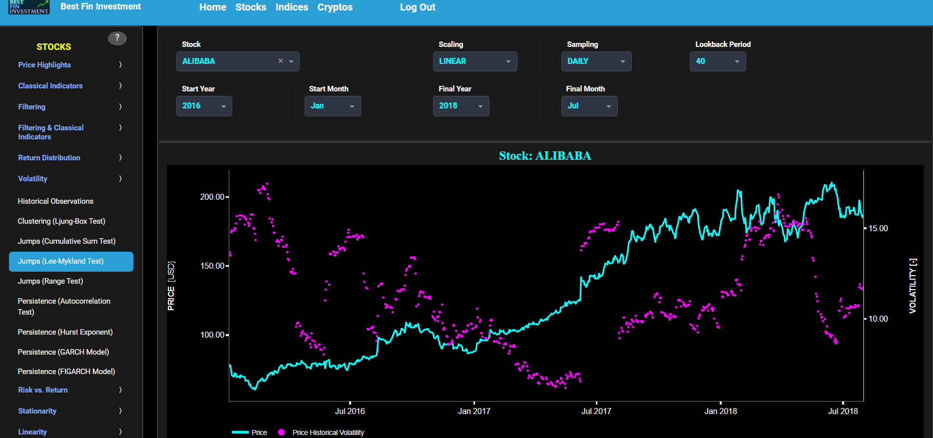
Jumps (Lee-Mykland Test)
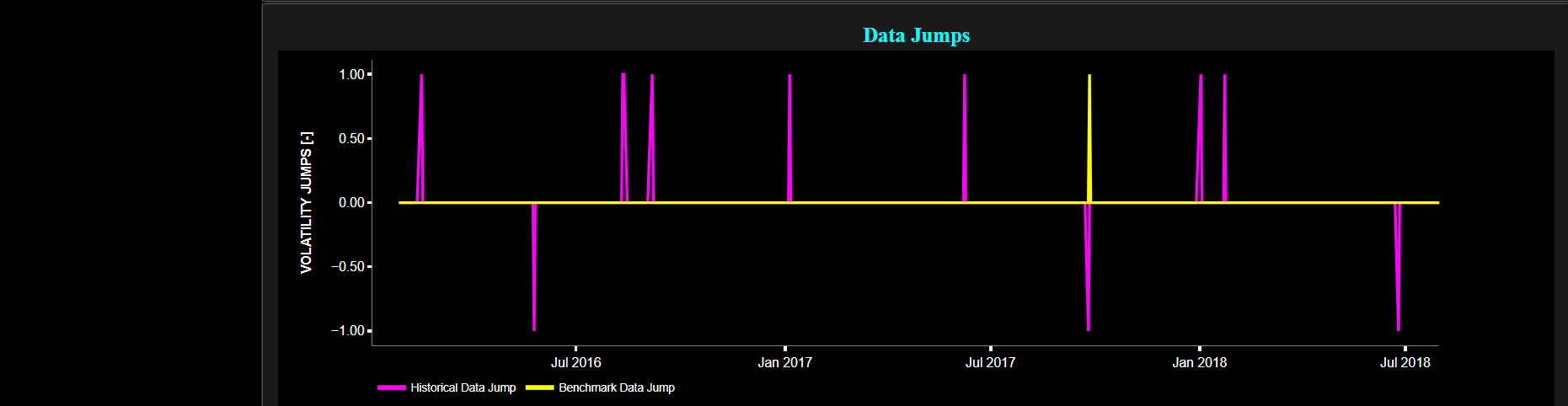
This page provides 3 graphs. The upper graph visualizes historical asset prices in cyan color using either daily, weekly, or monthly close prices. In the menu bar (located just above the graphs), you can also select specific time periods to visualize and also toggle between a linear or logarithmic price scaling on the left y-axis. Next to the cyan line, the upper graph also visualizes the historical asset volatility. This volatility is shown in magenta and expressed on the right y-axis. The volatility is computed using a lookback time period that is selected in the menu bar (located just above the graphs).
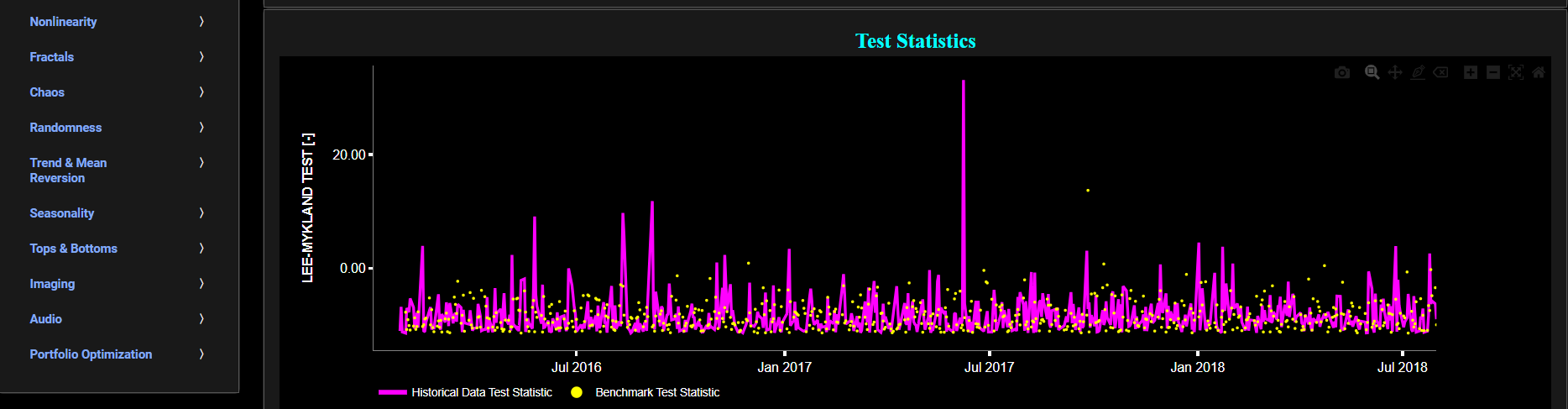
The middle graph visualizes the so-called “T” statistic for the Lee-Mykland (LM) test for the asset returns in magenta, and for a benchmark time series in yellow. This benchmark signal is based upon synthetically generated, normally distributed, independent and identically distributed (i.i.d.) returns. For this benchmark signal, each step is independent of the previous steps, and there is no systematic trend or pattern in the data. The yellow data points are given here for reference and comparison purposes (hence benchmarking). Now the LM statistical test is used to detect volatility jumps, particularly large and abrupt ones which are often associated with significant events, and the “T” test statistic summarizes the overall evidence for jumps in the time series. Note that in our case we have applied this test to the asset returns rather than asset volatility, as the algorithm has an internal volatility estimation procedure based upon a so-called rolling window realized bipower variation. Further we have also used this test with a 5% significance level threshold.
Finally the lower graph visualizes the so-called “J” Jump statistic for both the asset and benchmark signals. Here the convention reads as follows: J = 1 suggests an upward volatility jump, J = -1 suggests a downward volatility jump, and J = 0 indicates no significant volatility jump.
Volatility
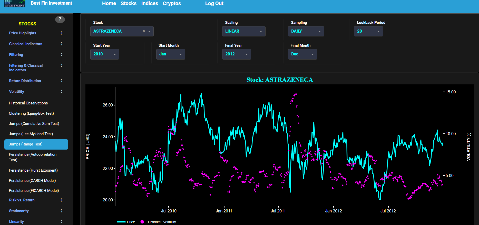
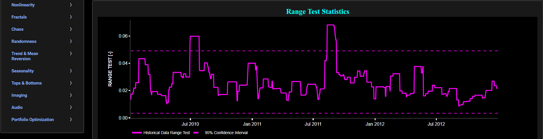
Jumps (Range Test)
This page provides 2 graphs. The upper graph visualizes historical asset prices in cyan color using either daily, weekly, or monthly close prices. In the menu bar (located just above the graphs), you can also select specific time periods to visualize and also toggle between a linear or logarithmic price scaling on the left y-axis. Next to the cyan line, the upper graph also visualizes the historical asset volatility. This volatility is shown in magenta and expressed on the right y-axis. The volatility is computed using a lookback time period that is selected in the menu bar (located just above the graphs). The lower graph visualizes the Range test statistic which is designed to quantify the magnitude or size of the jumps or fluctuations in financial data. It provides a measure of how significant or pronounced the jumps in the data are, which can be useful for identifying and characterizing volatility changes. The Range test is shown for the asset returns in magenta. Finally the dashed lines visualize the 95% confidence interval.
Volatility
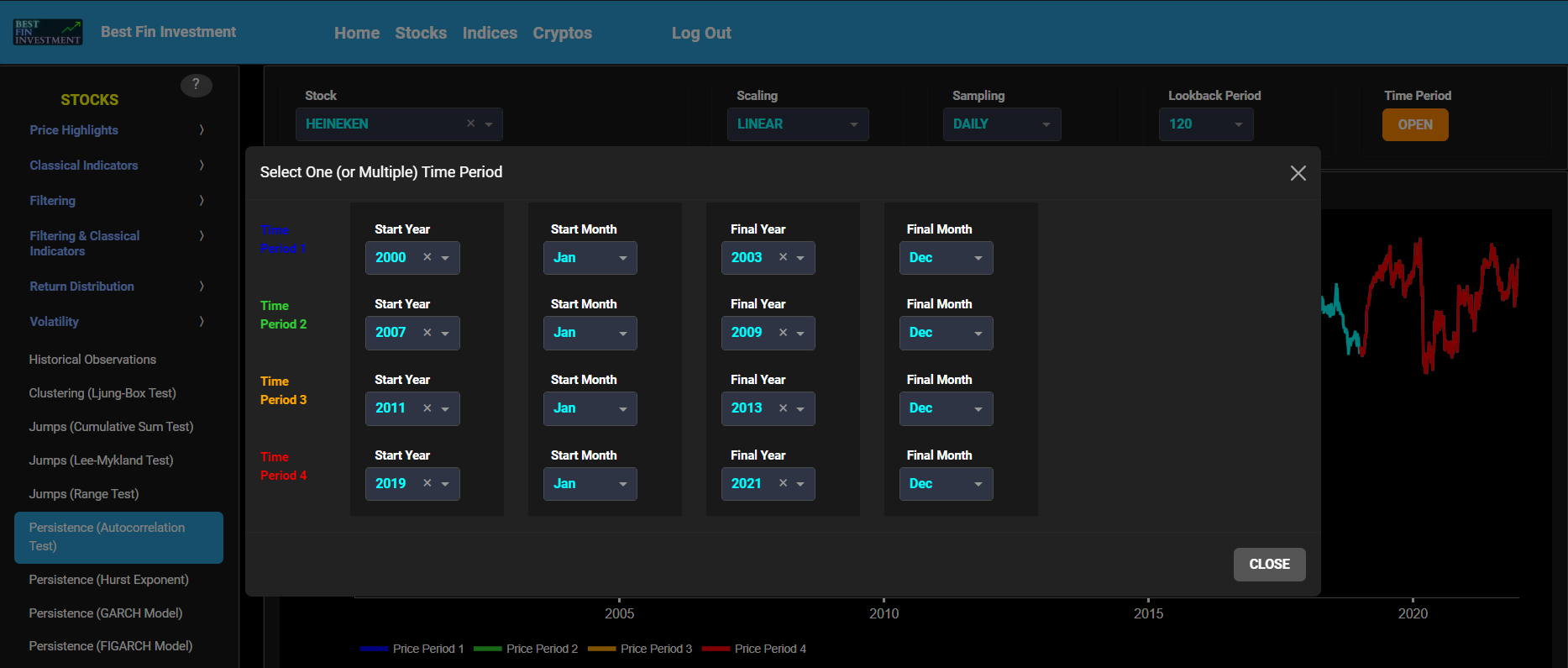
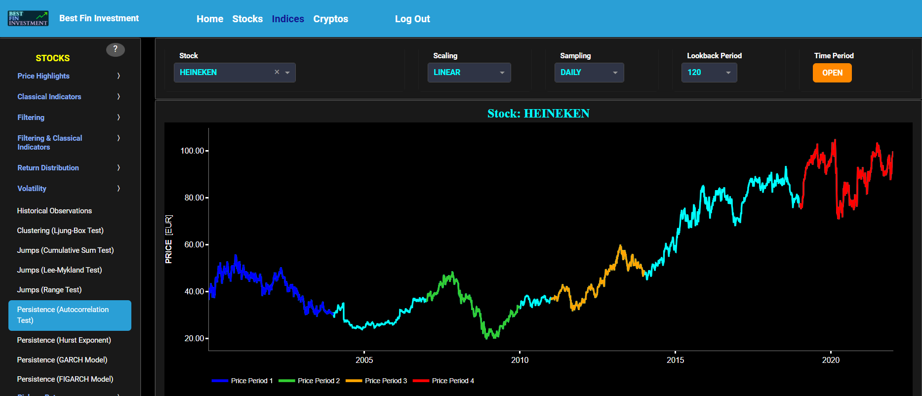
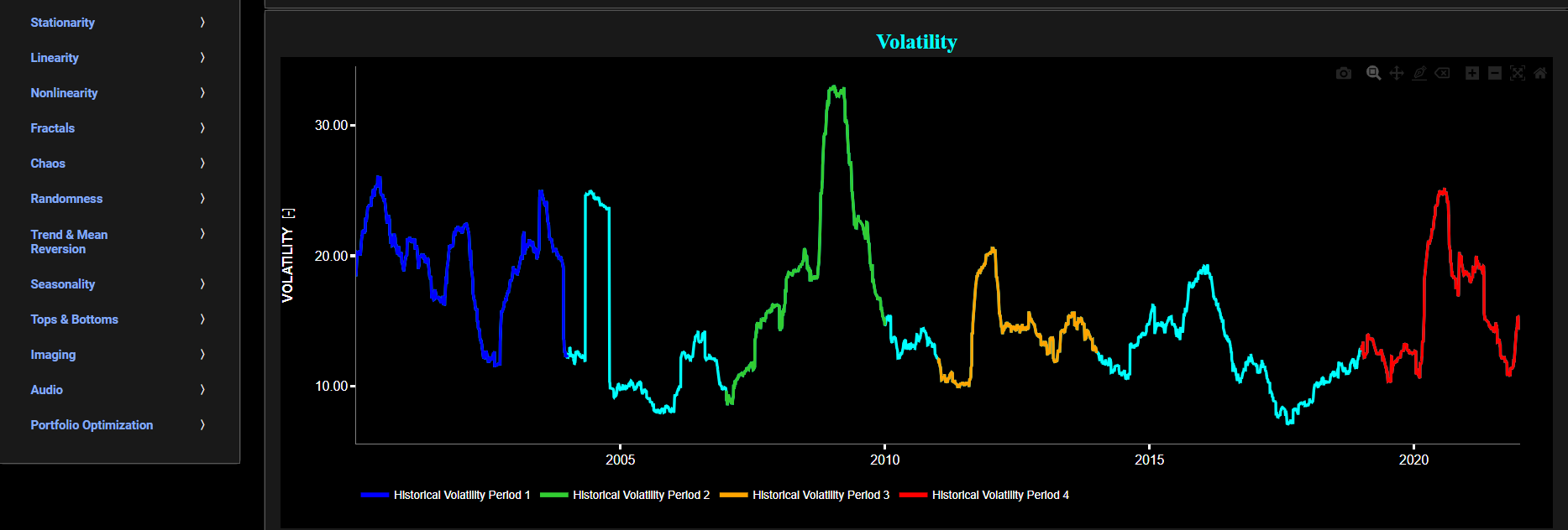
Persistence (Autocorrelation Test)
This page provides 3 graphs. The upper graph visualizes historical asset prices using either daily, weekly, or monthly close prices. In the menu bar (located just above the graphs), you can also toggle between a linear or logarithmic price scaling on the y-axis. Further you can select up to 4 specific time periods for further comparisons of price and volatility characteristics.
The middle graph visualizes the historical asset volatility. This volatility is shown for all selected time periods. The volatility is computed using a lookback time period that is selected in the menu bar (located just above the graphs).
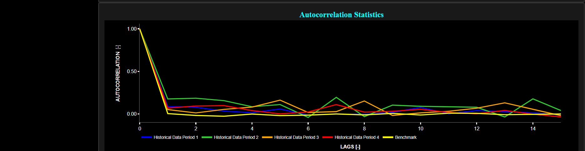
Finally the lower graph visualizes volatility persistence, i.e. high volatility persistence suggests that periods of high or low volatility tend to persist over time. Here we compute the Partial Autocorrelation Function (PACF) of the squared asset returns using a 95% confidence interval. Squaring the returns is a common practice when studying volatility because it amplifies the impact of extreme values, making volatility patterns more apparent. Specifically the PACF values measure the relationship between the squared returns at different lags, while controlling for the influence of shorter lags. Significant PACF values at longer lags may indeed indicate the presence of volatility persistence in the data, i.e. large PACF values at longer lags provide evidence of past volatility's influence on current volatility.
Note that the Autocorrelation Function (ACF) measures the relationship between a data point and its lagged values, including all shorter lags, whereas the PACF measures the relationship between a data point and its lagged values while controlling for the influence of shorter lags. Therefore the PACF is better suited for identifying the direct influence of a specific lag on the current data point. The PACF is shown separately for each selected time period and for a benchmark time series in yellow. This benchmark signal is based upon synthetically generated, normally distributed, independent and identically distributed (i.i.d.) returns. For this benchmark signal, each step is independent of the previous steps, and there is no systematic trend or pattern in the data. The yellow data points are given here for reference and comparison purposes (hence benchmarking).
Volatility
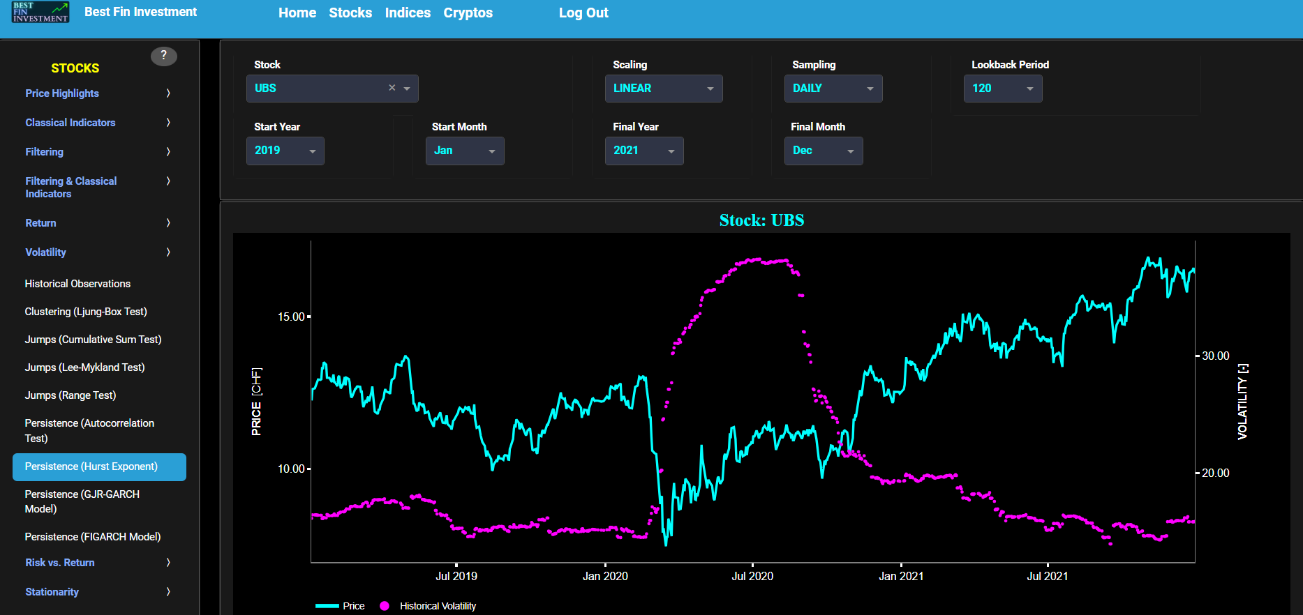
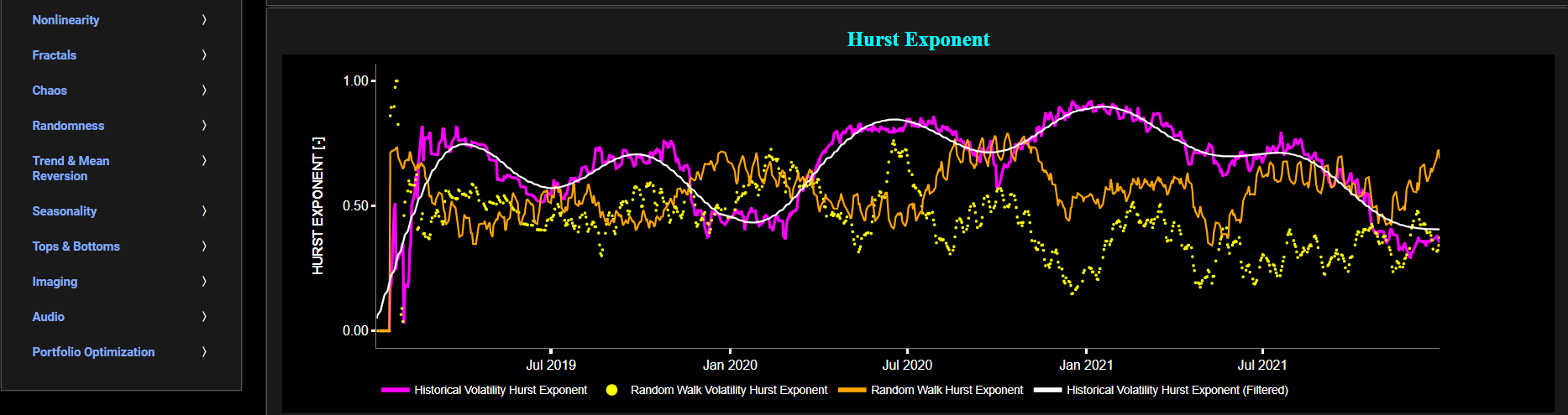
Persistence (Hurst Exponent)
This page provides 2 graphs. The upper graph visualizes historical asset prices in cyan color using either daily, weekly, or monthly close prices. In the menu bar (located just above the graphs), you can also select specific time periods to visualize and also toggle between a linear or logarithmic price scaling on the left y-axis. Next to the cyan line, the upper graph also visualizes the historical asset volatility. This volatility is shown in magenta and expressed on the right y-axis. The volatility is computed using a lookback time period that is selected in the menu bar (located just above the graphs).
The lower graph visualizes the Hurst Exponent (HE) statistical measure computed using the R/S statistic. The HE, named after the British hydrologist Harold Edwin Hurst (1880 – 1978), is used in various fields, including hydrology, to assess long-range dependence or persistence in time series data. In the context of hydrology, the HE is often used to analyze and understand the behavior of hydrological processes, particularly the flow of water in rivers, streams, and other water bodies. Essentially the HE helps to understand whether the flow at a particular time is influenced by past flow measurements over extended periods, i.e. the long-range dependence or memory of river flow. Similarly in financial time series analysis, the HE may be used to, among others, assess the persistence or long-term memory of asset volatility. It is particularly useful for understanding whether past volatility affects future volatility and for identifying patterns of persistence (such as persistence of trends) or mean-reverting behavior in financial markets. Here the HE is shown for the asset volatility in magenta, for a synthetically generated random walk in orange, and for the volatility of a random walk in yellow. In a random walk, each step is independent of the previous steps, and there is no systematic trend or pattern in the data. The random walk data points are given here for reference and comparison purposes (i.e. benchmarking). Next the white line represents a filtered version of the magenta line through the application of a low-pass Butterworth digital filter.
Finally the HE interpretation is given as follows: A HE value close to 0 suggests anti-persistence, where high volatility is likely to be followed by low volatility, and vice versa. A HE value close to 1 indicates persistence, where high volatility tends to be followed by high volatility, and low volatility by low volatility. A HE value around 0.5 suggests a random walk or no significant autocorrelation in volatility.
Volatility
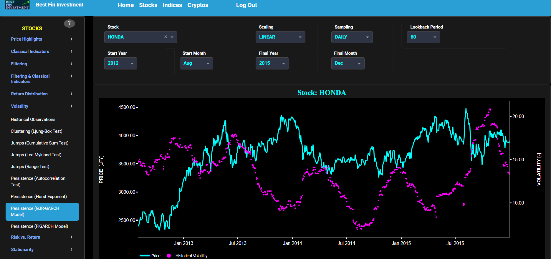
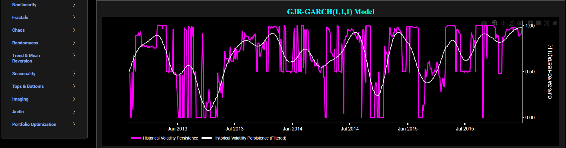
Persistence (GJR-GARCH Model)
This page provides 2 graphs. The upper graph visualizes historical asset prices in cyan color using either daily, weekly, or monthly close prices. In the menu bar (located just above the graphs), you can also select specific time periods to visualize and also toggle between a linear or logarithmic price scaling on the left y-axis. Next to the cyan line, the upper graph also visualizes the historical asset volatility. Here, volatility is defined as the annualized volatility of asset log returns. This volatility is shown in magenta and expressed on the right y-axis. The volatility is computed using a lookback time period that is selected in the menu bar (located just above the graphs).
The lower graph visualizes volatility persistence, i.e. the tendency of volatility to persist or autocorrelate over time. Here we use a Generalized Autoregressive Conditional Heteroskedasticity (GARCH) model which is commonly used in finance to model and forecast volatility. The basic GARCH model has been augmented with a so-called Generalized Jump Regression (GJR) term which allows to incorporate sudden jumps or shocks in volatility beyond what a standard GARCH model can capture. This means that the model can capture sudden changes in volatility due to unexpected events or shocks. Specifically the lower graph visualizes in magenta color the estimated model coefficient associated with the lagged conditional variance term (with lag 1). Next the white line represents a filtered version of the magenta line through the application of a low-pass Butterworth digital filter. Finally this graph may be interpreted as follows: if the shown coefficient values are close to 1, it suggests that past volatility has a strong influence on current volatility, indicating persistence. On the other hand if the shown coefficient values are significantly different from 1, it suggests that volatility may not exhibit strong persistence.
Volatility
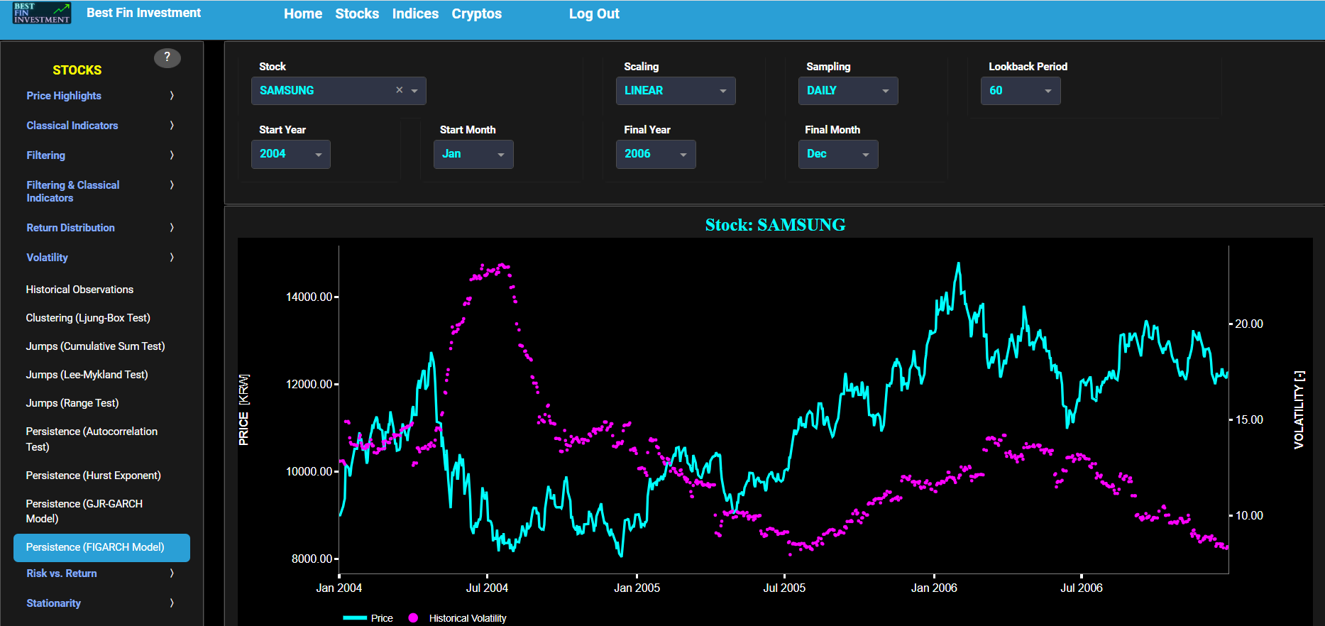
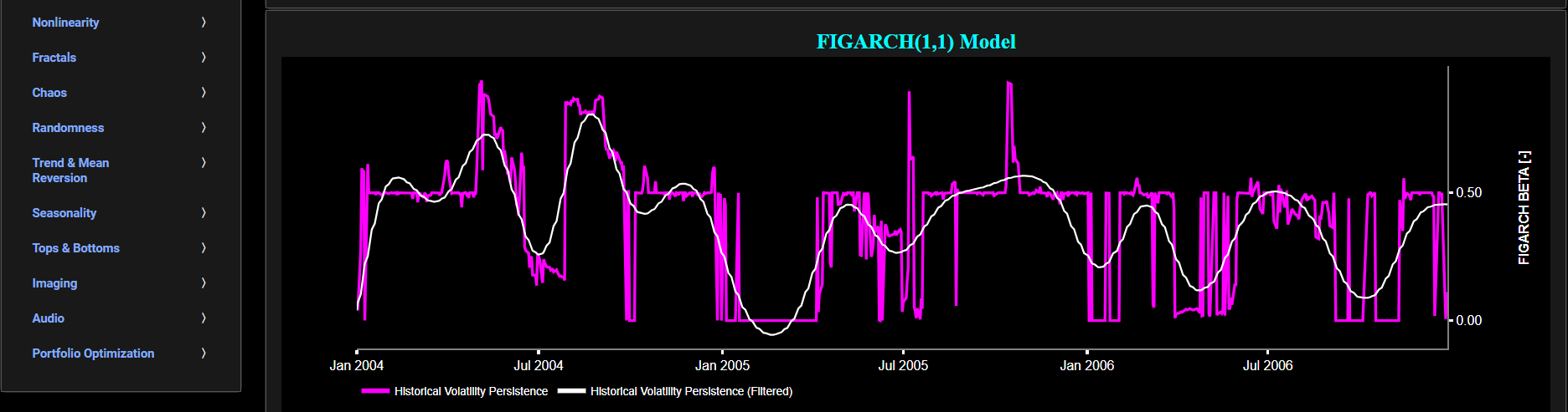
Persistence (FIGARCH Model)
This page provides 2 graphs. The upper graph visualizes historical asset prices in cyan color using either daily, weekly, or monthly close prices. In the menu bar (located just above the graphs), you can also select specific time periods to visualize and also toggle between a linear or logarithmic price scaling on the left y-axis. Next to the cyan line, the upper graph also visualizes the historical asset volatility. Here, volatility is defined as the annualized volatility of asset log returns. This volatility is shown in magenta and expressed on the right y-axis. The volatility is computed using a lookback time period that is selected in the menu bar (located just above the graphs).
The lower graph visualizes volatility persistence, i.e. the tendency of volatility to persist or autocorrelate over time. Here we use a Fractionally Integrated Generalized Autoregressive Conditional Heteroskedasticity (FIGARCH) model, whose primary focus is on capturing long memory or long-range dependence in volatility (typically associated with autocorrelation in the squared asset returns). The FIGARCH model achieves this by including a so-called fractional differencing parameter to account for the persistence in volatility. Specifically the lower graph visualizes in magenta color this estimated fractional differencing parameter. Essentially this parameter controls how quickly past shocks in volatility decay over time. A higher parameter value leads to slower decay and higher persistence, while a lower parameter value leads to faster decay and lower persistence. Next the white line represents a filtered version of the magenta line through the application of a low-pass Butterworth digital filter. Finally this graph may be interpreted as follows. A value close to 1 suggests high persistence in volatility. It indicates that past volatility strongly influences current volatility, and there is a significant autocorrelation in the squared asset returns. In this case, volatility tends to persist over time. On the other hand a value close to 0 indicates low persistence or near-random walk behavior in volatility. It suggests that past volatility does not have a strong influence on current volatility, and there is little autocorrelation in the squared asset returns. Finally an intermediate value suggests moderate persistence. It implies that past volatility has a moderate influence on current volatility, and there is some autocorrelation in the squared asset returns.
Risk vs. Return
Animation
This page visualizes asset “Risk” versus “Return”, through a video animation, using either daily, weekly, or monthly close prices. In the menu bar (located just above the graph), you can also select specific time periods to visualize. Here “Risk” is defined as the annualized sample volatility of the financial asset's returns based upon the lookback time period. It is a measure of how much the returns vary over time, scaled to an annualized basis. The lookback time period can also be selected from the menu bar (located just above the graph). Next “Return” is here defined as the percentage change in price from one time period to the next and subsequently averaged over the lookback time period. Now clicking on the orange “PLAY” button will start the video animation. The main purpose of this animation is to get a sense of market cycles and their associated clockwise or counter-clockwise rotations.

Risk vs. Return
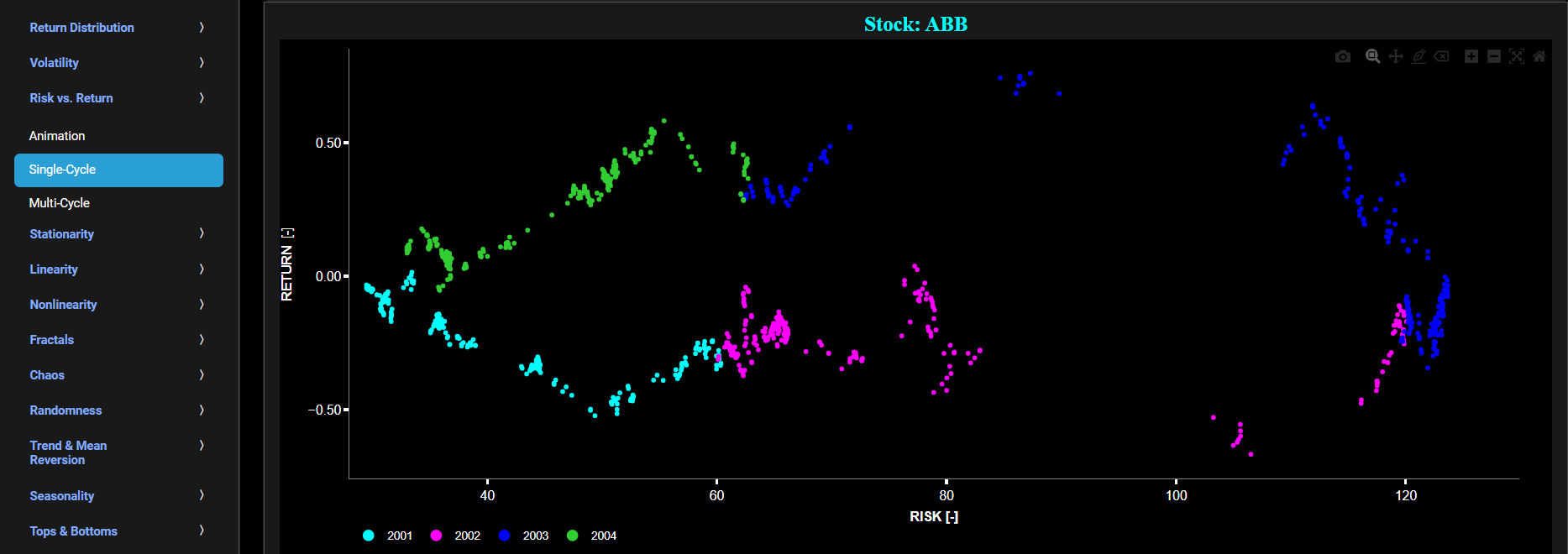
Single-Cycle
This page visualizes asset “Risk” versus “Return”, in a single graph, using either daily, weekly, or monthly close prices. In the menu bar (located just above the graph), you can also select specific time periods to visualize. Here “Risk” is defined as the annualized sample volatility of the financial asset's returns based upon the lookback time period. It is a measure of how much the returns vary over time, scaled to an annualized basis. The lookback time period can also be selected from the menu bar (located just above the graph). Next “Return” is here defined as the percentage change in price from one time period to the next and subsequently averaged over the lookback time period. On this graph each year will be shown with a different color coding, hence helping you identify market cycles and their associated clockwise or counter-clockwise rotations.

Risk vs. Return
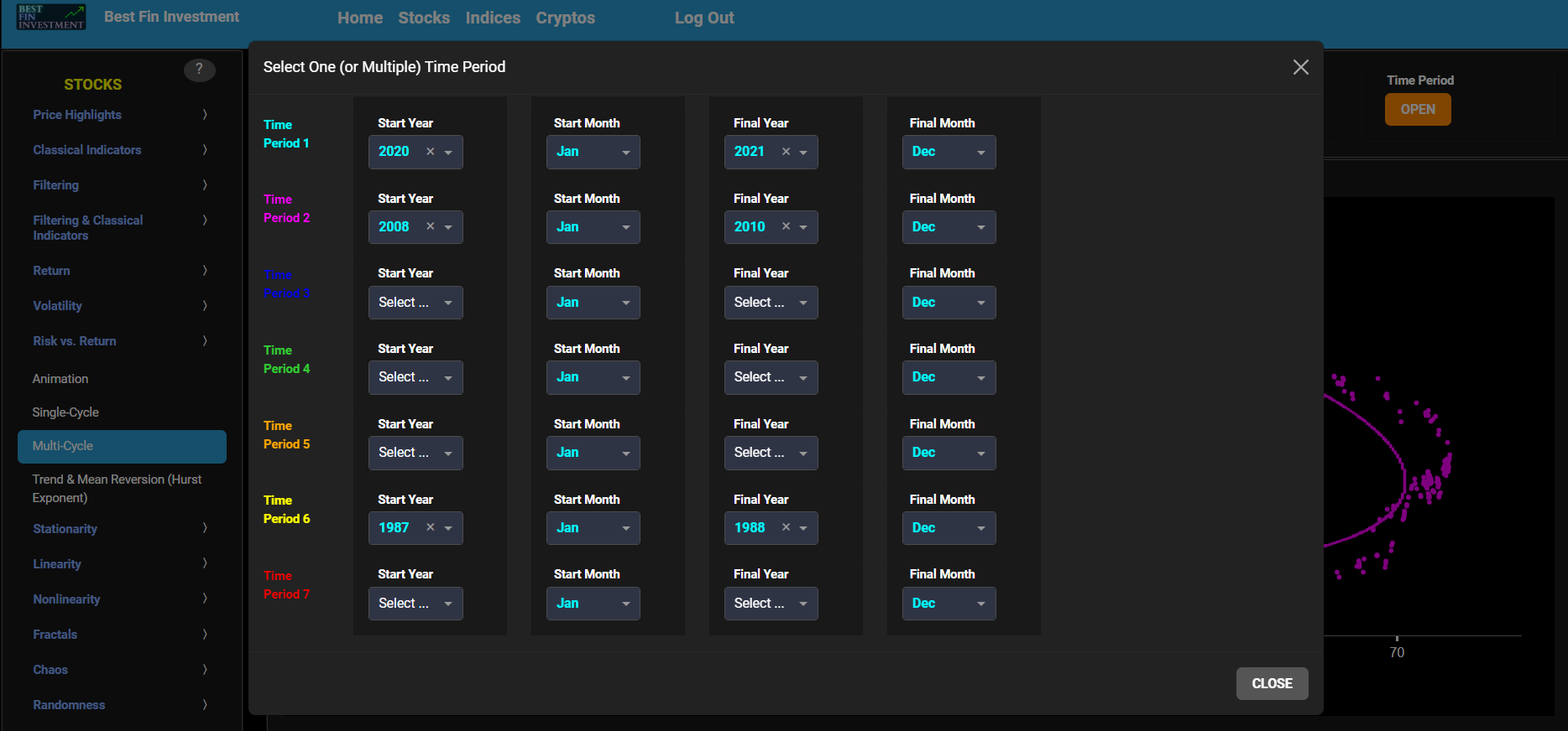
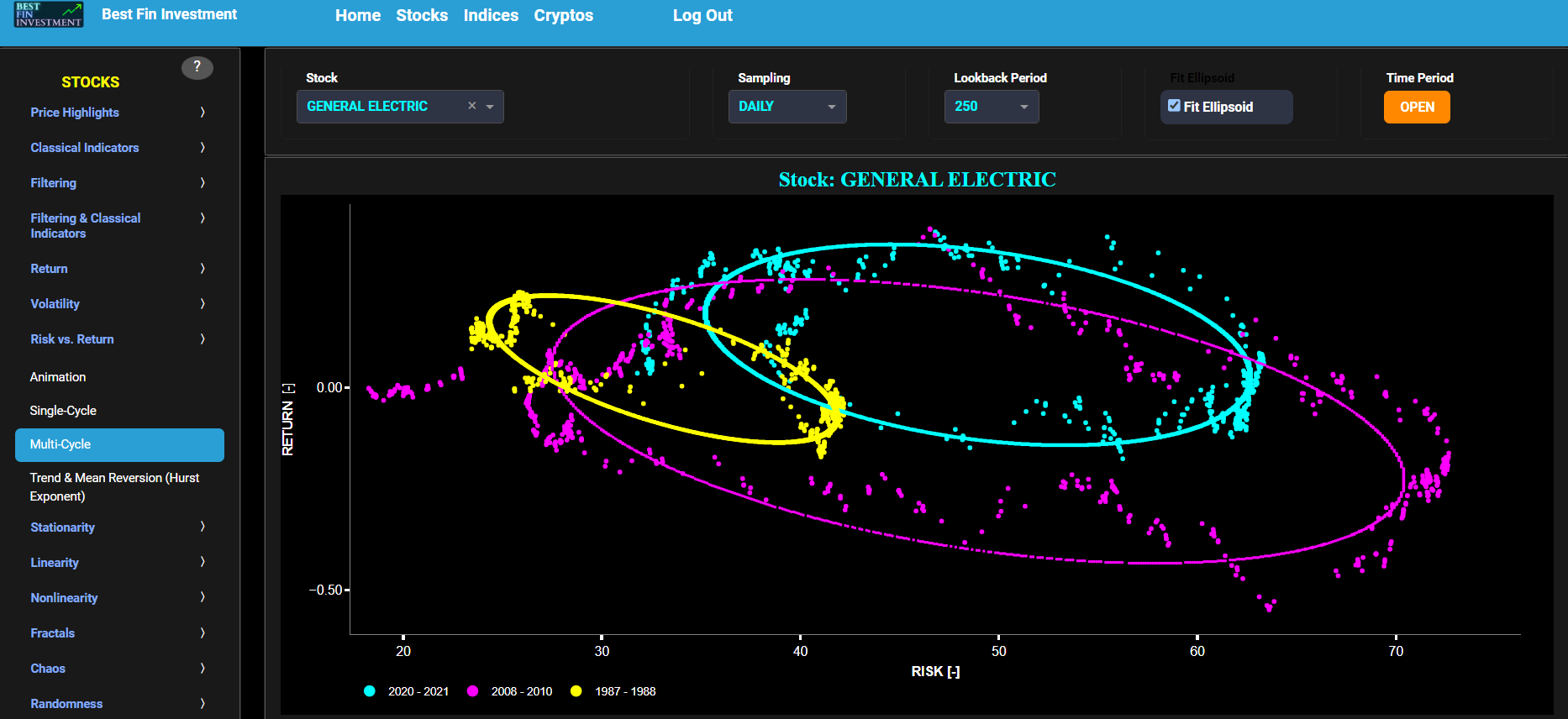
Multi-Cycle
This page visualizes asset “Risk” versus “Return”, in a single graph, using either daily, weekly, or monthly close prices. In the menu bar (located just above the graph), you can also select up to 4 specific time periods for comparisons (each having its own color). Here “Risk” is defined as the annualized sample volatility of the financial asset's returns based upon the lookback time period. It is a measure of how much the returns vary over time, scaled to an annualized basis. The lookback time period can also be selected from the menu bar (located just above the graph). Next “Return” is here defined as the percentage change in price from one time period to the next and subsequently averaged over the lookback time period. On this graph each time period will be shown with a different color coding, hence helping you compare the various market cycles. Finally you can also add an ellipsoid fit to all shown market cycles, using a toggle button available on the menu bar.
Risk vs. Return
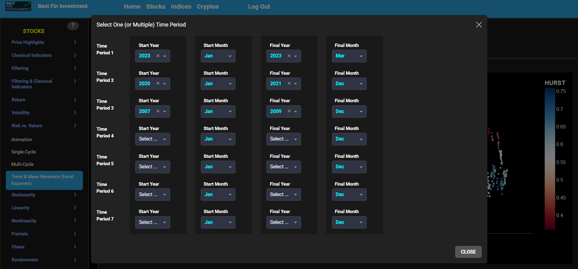
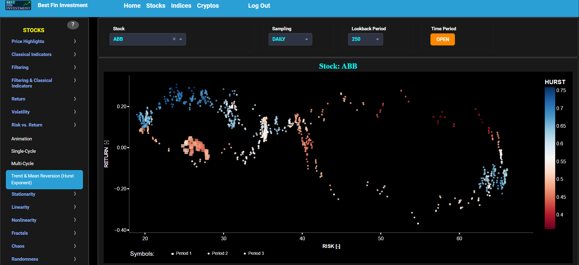
Trend & Mean Reversion (Hurst Exponent)
This page visualizes asset “Risk” versus “Return” with the Hurst Exponent (HE) as color coding using either daily, weekly, or monthly close prices. In the menu bar (located just above the graph), you can also select up to 2 specific time periods for comparisons. Here “Risk” is defined as the annualized sample volatility of the financial asset's returns based upon the lookback time period. It is a measure of how much the returns vary over time, scaled to an annualized basis. The lookback time period can also be selected from the menu bar (located just above the graph). Next “Return” is defined as the percentage change in price from one time period to the next and subsequently averaged over the lookback time period.
In our case the HE statistical measure is computed using the R/S statistic. The HE, named after the British hydrologist Harold Edwin Hurst (1880 – 1978), is used in various fields, including hydrology, to assess long-range dependence or persistence in time series data. In the context of hydrology, the HE is often used to analyze and understand the behavior of hydrological processes, particularly the flow of water in rivers, streams, and other water bodies. Essentially the HE helps to understand whether the flow at a particular time is influenced by past flow measurements over extended periods, i.e. the long-range dependence or memory of river flow. Similarly in financial time series analysis, the HE may be used to analyze the intrinsic behavior of the asset's price movements. When applied to asset prices, the HE helps analyze whether the asset's prices exhibit a trending (persistent) or ean-reverting (anti-persistent) behavior. Here the HE is computed using the lookback time period that is selected in the menu bar (located just above the graph).
In terms of HE interpretation we have the following: A HE < 0.5 indicates a mean-reverting or anti-persistent behavior. In the context of asset prices, it suggests that the asset tends to revert to its mean price over time. This could imply opportunities for contrarian strategies. A HE > 0.5 suggests a trending or persistent behavior, indicating that the asset exhibits long-term trends and momentum. A HE value around 0.5 suggests a random walk.
Stationarity
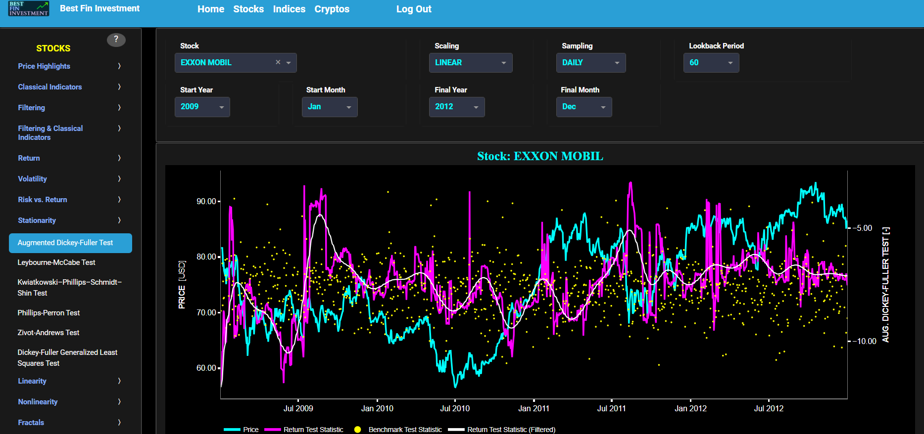
Augmented Dickey-Fuller Test
This page provides 2 graphs. The upper graph visualizes historical asset prices in cyan color using either daily, weekly, or monthly close prices. In the menu bar (located just above the graphs), you can also select specific time periods to visualize and also toggle between a linear or logarithmic price scaling on the y-axis. Next to the cyan line, the upper graph also visualizes the test statistic for the Augmented Dickey-Fuller (ADF) test for the asset incremental returns in magenta, and for a benchmark time series in yellow. This benchmark signal is based upon synthetically generated, normally distributed, independent and identically distributed (i.i.d.) returns. For this benchmark signal, each step is independent of the previous steps, and there is no systematic trend or pattern in the data. The yellow data points are given here for reference and comparison purposes (hence benchmarking). Next the white line represents a filtered version of the magenta line through the application of a low-pass Butterworth digital filter.
In our case the ADF test is applied using a constant (intercept) and a trend component when testing for stationarity of the asset returns. When a time series is non-stationary (i.e. it has a so-called unit root) it means that it exhibits a stochastic trend or a non-constant mean over time. In other words, the statistical properties of the time series, such as the mean and variance, are not constant over time. Here the null hypothesis of the ADF test is that the time series has a unit root, which means it is non-stationary. The alternative hypothesis is that the time series is stationary, i.e. it does not have a unit root. Now if the test statistic is significantly different from 0, it suggests evidence against the null hypothesis. In other words, it indicates that the time series is likely stationary, as it does not exhibit a unit root. Conversely if the test statistic is close to 0, it means that there is not enough evidence to reject the null hypothesis. In this case, the time series is more likely to be non-stationary, indicating the presence of a unit root.
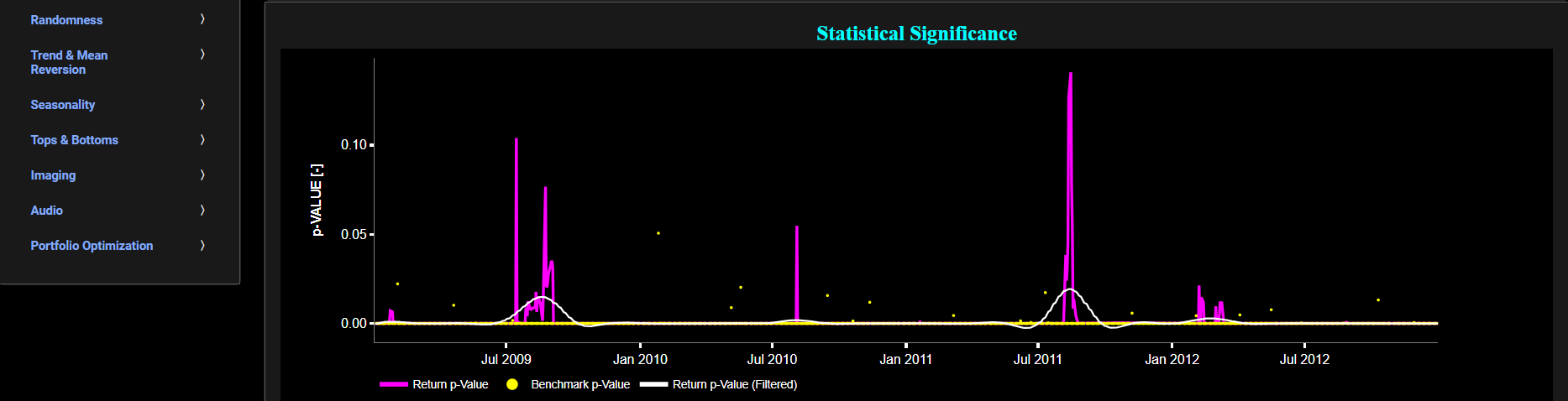
Next the lower graph visualizes the statistical significance (or so called p-value) for the ADF test and for the benchmark signal. If the p-value is less than a significance level (typically 0.05), we may reject the null hypothesis and conclude that the data is stationary. Otherwise, if the p-value is greater than the significance level, we may fail to reject the null hypothesis, hence indicating non-stationarity. Finally in the menu bar (located just above the graphs), you can also select specific values for the lookback time period on which the ADF test will be computed.
Stationarity
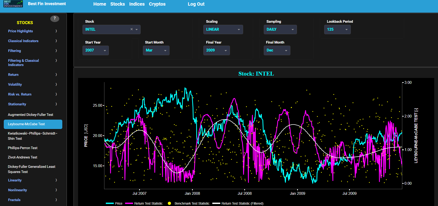
Leybourne-McCabe Test
This page provides 2 graphs. The upper graph visualizes historical asset prices in cyan color using either daily, weekly, or monthly close prices. In the menu bar (located just above the graphs), you can also select specific time periods to visualize and also toggle between a linear or logarithmic price scaling on the y-axis. Next to the cyan line, the upper graph also visualizes the test statistic for the Leybourne-McCabe (LM) test for the asset cumulative returns in magenta, and for a synthetically generated random walk in yellow. In a random walk, each step is independent of the previous steps, and there is no systematic trend or pattern in the data. The yellow random walk data points are given here for reference and comparison purposes (i.e. benchmarking). Next the white line represents a filtered version of the magenta line through the application of a low-pass Butterworth digital filter.
In our case the LM test is applied using a constant (intercept) and a trend component when testing for stationarity of the asset returns. When a time series is non-stationary (i.e. it has a so-called unit root) it means that it exhibits a stochastic trend or a non-constant mean over time. In other words, the statistical properties of the time series, such as the mean and variance, are not constant over time. Here the null hypothesis of the LM test is that the time series is stationary. The alternative hypothesis is that the time series is non-stationary, i.e. it does have a unit root. Now if the test statistic is significantly different from 0, it suggests evidence against the null hypothesis. In other words, it indicates that the time series is likely non-stationary, as it does exhibit a unit root. Conversely if the test statistic is close to 0, it means that there is not enough evidence to reject the null hypothesis. In this case, the time series is more likely to be stationary.
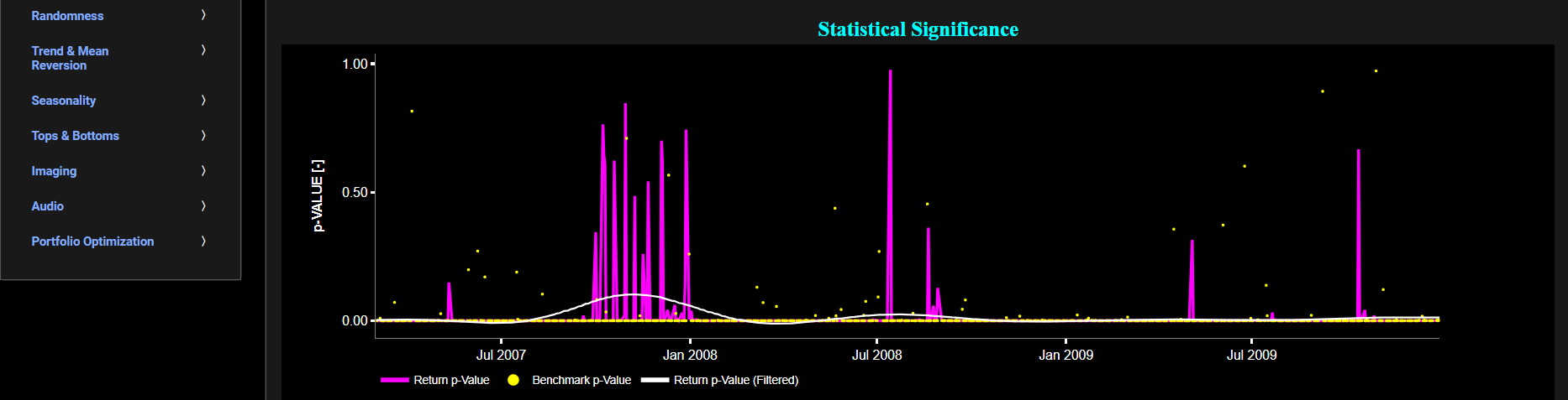
Next the lower graph visualizes the statistical significance (or so called p-value) for the LM test and for the benchmark signal. If the p-value is less than a significance level (typically 0.05), we may reject the null hypothesis and conclude that the data is non-stationary. Otherwise, if the p-value is greater than the significance level, we may fail to reject the null hypothesis, hence indicating stationarity. Finally in the menu bar (located just above the graphs), you can also select specific values for the lookback time period on which the LM test will be computed.
Stationarity
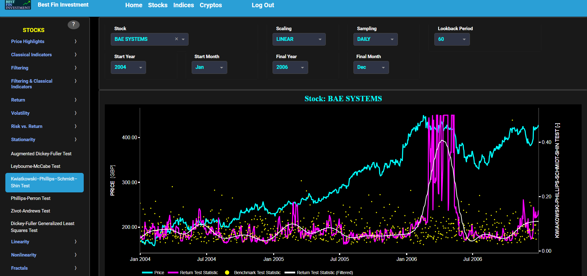
Kwiatkowski–Phillips–Schmidt–Shin Test
This page provides 2 graphs. The upper graph visualizes historical asset prices in cyan color using either daily, weekly, or monthly close prices. In the menu bar (located just above the graphs), you can also select specific time periods to visualize and also toggle between a linear or logarithmic price scaling on the y-axis. Next to the cyan line, the upper graph also visualizes the test statistic for the Kwiatkowski–Phillips–Schmidt–Shin (KPSS) test for the asset incremental returns in magenta, and for a benchmark time series in yellow. This benchmark signal is based upon synthetically generated, normally distributed, independent and identically distributed (i.i.d.) returns. For this benchmark signal, each step is independent of the previous steps, and there is no systematic trend or pattern in the data. The yellow data points are given here for reference and comparison purposes (hence benchmarking). Next the white line represents a filtered version of the magenta line through the application of a low-pass Butterworth digital filter.
In our case the KPSS test is applied using a constant (intercept) and a trend component when testing for stationarity of the asset returns. When a time series is non-stationary (i.e. it has a so-called unit root) it means that it exhibits a stochastic trend or a non-constant mean over time. In other words, the statistical properties of the time series, such as the mean and variance, are not constant over time. Here the null hypothesis for the KPSS test is that the time series data is stationary around a deterministic trend. In other words, the null hypothesis assumes that the data is stationary with a constant mean and variance but may have a linear trend. The alternative hypothesis is that the time series is non-stationary, meaning it has a unit root, a stochastic trend, or some other form of non-constant variance. Now if the test statistic is significantly different from 0 (i.e. far from 0 by exceeding critical values), it suggests that the time series has a unit root, indicating non-stationarity. In this case, you may reject the null hypothesis (i.e., you conclude that the data is non-stationary). Conversely if the test statistic is close to 0, it suggests that the time series is stationary around a deterministic trend. In this case, you fail to reject the null hypothesis (i.e., you conclude that the data is stationary).
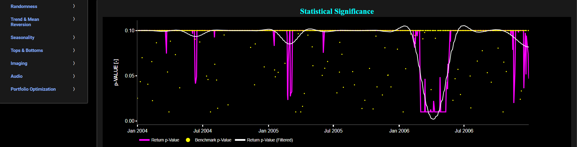
Next the lower graph visualizes the statistical significance (or so called p-value) for the KPSS test and for the benchmark signal. A low p-value (typically less than 0.05) suggests that the data is non-stationary, as you would reject the null hypothesis. A high p-value suggests that the data is stationary, as you fail to reject the null hypothesis. Finally in the menu bar (located just above the graphs), you can also select specific values for the lookback time period on which the KPSS test will be computed.
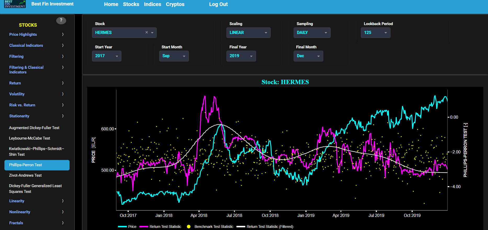
Stationarity
Phillips-Perron Test
This page provides 2 graphs. The upper graph visualizes historical asset prices in cyan color using either daily, weekly, or monthly close prices. In the menu bar (located just above the graphs), you can also select specific time periods to visualize and also toggle between a linear or logarithmic price scaling on the y-axis. Next to the cyan line, the upper graph also visualizes the test statistic for the Phillips-Perron (PP) test for the asset cumulative returns in magenta, and for a synthetically generated random walk in yellow. In a random walk, each step is independent of the previous steps, and there is no systematic trend or pattern in the data. The yellow random walk data points are given here for reference and comparison purposes (i.e. benchmarking). Next the white line represents a filtered version of the magenta line through the application of a low-pass Butterworth digital filter.
In our case the PP test is applied using a constant (intercept) and a trend component when testing for stationarity of the asset returns. When a time series is non-stationary (i.e. it has a so-called unit root) it means that it exhibits a stochastic trend or a non-constant mean over time. In other words, the statistical properties of the time series, such as the mean and variance, are not constant over time. Here the null hypothesis of the PP test is that the time series has a unit root, which means it is non-stationary. The alternative hypothesis is that the time series is stationary, i.e. it does not have a unit root. Now if the test statistic is significantly different from 0 (i.e. far from 0 by exceeding critical values), it suggests evidence against the null hypothesis. In other words, it indicates that the time series is likely stationary, as it does not exhibit a unit root. Conversely if the test statistic is close to 0, it means that there is not enough evidence to reject the null hypothesis. In this case, the time series is more likely to be non-stationary, indicating the presence of a unit root.
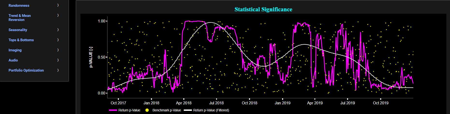
Next the lower graph visualizes the statistical significance (or so called p-value) for the PP test and for the benchmark signal. If the p-value is less than a significance level (typically 0.05), we may reject the null hypothesis and conclude that the data is stationary. Otherwise, if the p-value is greater than the significance level, we may fail to reject the null hypothesis, hence indicating non-stationarity. Finally in the menu bar (located just above the graphs), you can also select specific values for the lookback time period on which the PP test will be computed.
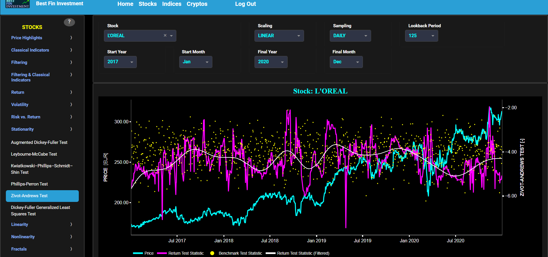
Stationarity
Zivot-Andrews Test
This page provides 2 graphs. The upper graph visualizes historical asset prices in cyan color using either daily, weekly, or monthly close prices. In the menu bar (located just above the graphs), you can also select specific time periods to visualize and also toggle between a linear or logarithmic price scaling on the y-axis. Next to the cyan line, the upper graph also visualizes the test statistic for the Zivot-Andrews (ZA) test for the asset cumulative returns in magenta, and for a synthetically generated random walk in yellow. In a random walk, each step is independent of the previous steps, and there is no systematic trend or pattern in the data. The yellow random walk data points are given here for reference and comparison purposes (i.e. benchmarking). Next the white line represents a filtered version of the magenta line through the application of a low-pass Butterworth digital filter.
In our case the ZA test is applied using a constant (intercept) and a trend component when testing for stationarity of the asset returns. Note that this test does allow for the possibility of a single structural break in the time series, which means that the characteristics of the series may have changed at some point. When a time series is non-stationary (i.e. it has a so-called unit root) it means that it exhibits a stochastic trend or a non-constant mean over time. In other words, the statistical properties of the time series, such as the mean and variance, are not constant over time. Here the null hypothesis of the ZA test is that the time series has a unit root, which means it is non-stationary. The alternative hypothesis is that the time series is stationary, i.e. it does not have a unit root. Now if the test statistic is significantly different from 0 (i.e. far from 0 by exceeding critical values), it suggests evidence against the null hypothesis. In other words, it indicates that the time series is likely stationary, as it does not exhibit a unit root. Conversely if the test statistic is close to 0, it means that there is not enough evidence to reject the null hypothesis. In this case, the time series is more likely to be non-stationary, indicating the presence of a unit root.
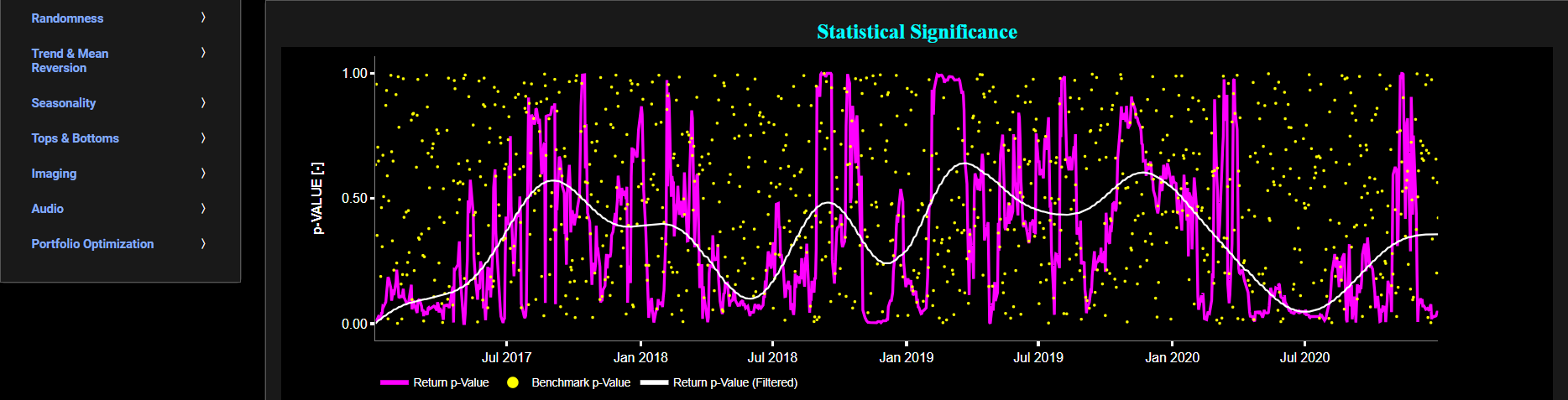
Next the lower graph visualizes the statistical significance (or so called p-value) for the ZA test and for the benchmark signal. If the p-value is less than a significance level (typically 0.05), we may reject the null hypothesis and conclude that the data is stationary. Otherwise, if the p-value is greater than the significance level, we may fail to reject the null hypothesis, hence indicating non-stationarity. Finally in the menu bar (located just above the graphs), you can also select specific values for the lookback time period on which the ZA test will be computed.
Stationarity
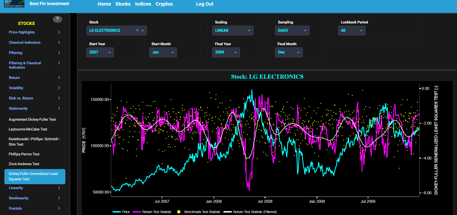
Dickey-Fuller Generalized Least Squares Test
This page provides 2 graphs. The upper graph visualizes historical asset prices in cyan color using either daily, weekly, or monthly close prices. In the menu bar (located just above the graphs), you can also select specific time periods to visualize and also toggle between a linear or logarithmic price scaling on the y-axis. Next to the cyan line, the upper graph also visualizes the test statistic for the Dickey-Fuller Generalized Least Squares (DFGLS) test for the asset cumulative returns in magenta, and for a synthetically generated random walk in yellow. In a random walk, each step is independent of the previous steps, and there is no systematic trend or pattern in the data. The yellow random walk data points are given here for reference and comparison purposes (i.e. benchmarking). Next the white line represents a filtered version of the magenta line through the application of a low-pass Butterworth digital filter.
In our case the DF-GLS test is applied using a constant (intercept) and a trend component when testing for stationarity of the asset returns. The DF-GLS test is a specialized modification of the Augmented Dickey-Fuller (ADF) test that may be chosen when serial correlation is a concern. The DF-GLS test is particularly useful when dealing with time series data that may exhibit serial correlation, which can lead to inaccurate results in standard unit root tests like the original Dickey-Fuller test. By using Generalized Least Squares, the DF-GLS test provides more robust results under such conditions. Now when a time series is non-stationary (i.e. it has a so-called unit root) it means that it exhibits a stochastic trend or a non-constant mean over time. In other words, the statistical properties of the time series, such as the mean and variance, are not constant over time. Here the null hypothesis of the DF-GLS test is that the time series has a unit root, which means it is non-stationary. The alternative hypothesis is that the time series is stationary, i.e. it does not have a unit root. Now if the test statistic is significantly different from 0, it suggests evidence against the null hypothesis. In other words, it indicates that the time series is likely stationary, after accounting for potential serial correlation and a deterministic trend component. Conversely if the test statistic is close to 0, it means that there is not enough evidence to reject the null hypothesis. In this case, the time series is more likely to be non-stationary, indicating the presence of a unit root.
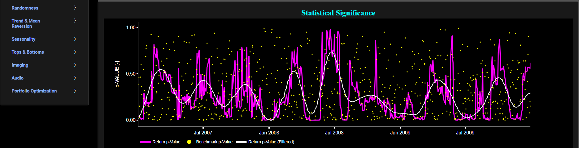
Next the lower graph visualizes the statistical significance (or so called p-value) for the DF-GLS test and for the benchmark signal. If the p-value is less than a significance level (typically 0.05), we may reject the null hypothesis and conclude that the data is stationary. Otherwise, if the p-value is greater than the significance level, we may fail to reject the null hypothesis, hence indicating non-stationarity. Finally in the menu bar (located just above the graphs), you can also select specific values for the lookback time period on which the DF-GLS test will be computed.
Linearity
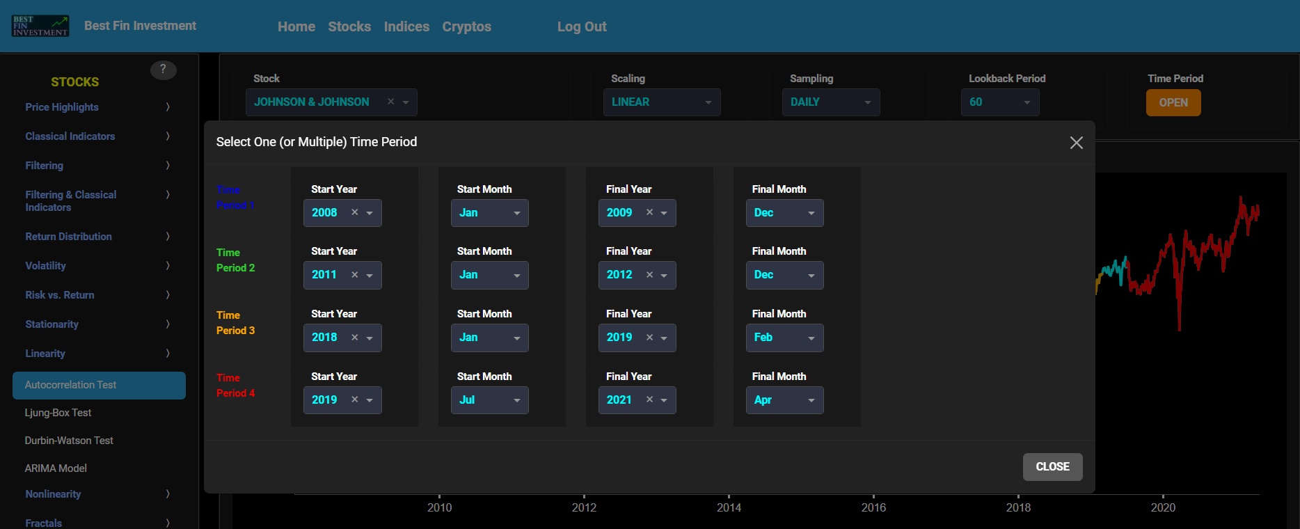
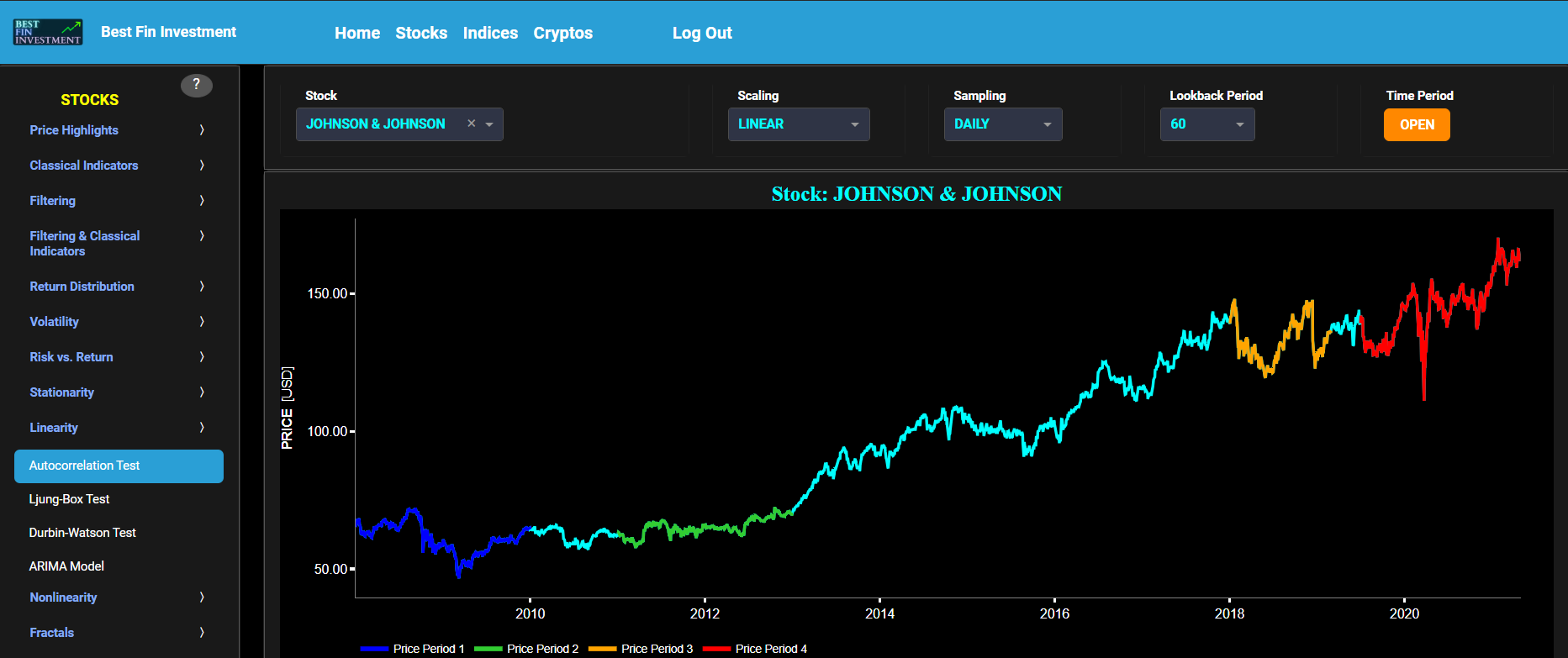
Autocorrelation Test
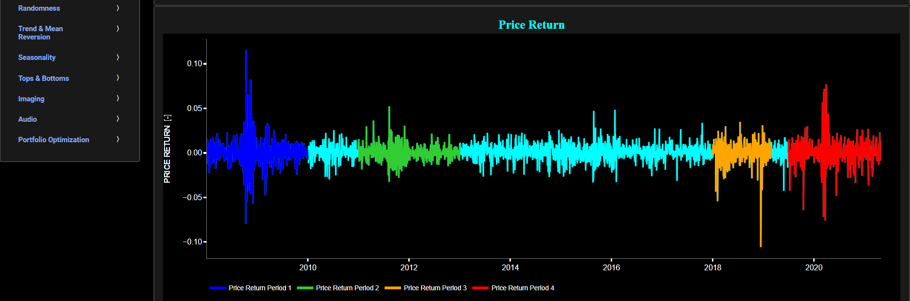
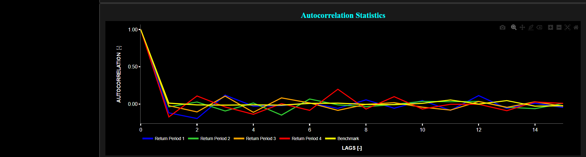
This page provides 3 graphs. The upper graph visualizes historical asset prices using either daily, weekly, or monthly close prices. In the menu bar (located just above the graphs), you can also toggle between a linear or logarithmic price scaling on the y-axis. Further you can select up to 4 specific time periods for further comparisons of price and return characteristics. The middle graph visualizes the historical asset return, with asset “return” defined as incremental returns (i.e. quantified as the percentage change in the asset's price between consecutive time periods). These asset returns are shown for all selected time periods using dedicated colors. Finally the lower graph analyzes the asset returns through the autocorrelation statistic. Indeed the autocorrelation is a valuable tool in time series analysis. Positive autocorrelation can indicate trends or seasonality, while negative autocorrelation might suggest a pattern of oscillation or inverse behavior in the data. The magnitude of the autocorrelation value indicates the strength of the relationship, with larger absolute values indicating a stronger relationship.
In our case we visualize the Partial Autocorrelation Function (PACF) of asset returns. The PACF is computed using a lookback time period that is selected in the menu bar (located just above the graphs). While the standard Autocorrelation Function (ACF) measures the relationship between a data point and its lagged values (including all shorter lags), the PACF measures the relationship between a data point and its lagged values while controlling for the influence of shorter lags. Therefore the PACF is better suited for identifying the direct influence of a specific lag on the current data point. Now when it comes to ACF or PACF metrics it is important to recognize the following characteristics. First, linear patterns in data can result in significant autocorrelation in the ACF and PACF plots. Hence a linear pattern is a sufficient condition for observing autocorrelation. Conversely the absence of autocorrelation guarantees the absence of linear patterns in the data. However non-linear patterns in data can also lead to autocorrelation. For instance, if a time series follows a periodic or cyclic pattern, it may exhibit autocorrelation at specific lags. Therefore, the presence of autocorrelation does not necessarily imply a linear pattern; it can also indicate non-linear dependencies (particularly when these patterns manifest themselves as spikes or oscillations in the PACF). Note that although the PACF may detect nonlinear behavior in the data, it is generally not as robust or specific as dedicated nonlinear time series analysis. Finally the absence of significant autocorrelation in the ACF or PACF does not necessarily mean that there are no non-linear patterns in the data. Non-linear patterns may not produce strong autocorrelation in these plots, especially if they are complex or irregular. Summarizing: while linear patterns will always lead to autocorrelation in ACF and PACF plots, non-linear patterns in the data may or may not lead to autocorrelation, depending on whether they involve systematic relationships between data points at different lags.
Now returning to the graphs, the lower graph also includes a benchmark time series in yellow. This benchmark signal is based upon synthetically generated, normally distributed, independent and identically distributed (i.i.d.) returns. For this benchmark signal, each step is independent of the previous steps, and there is no systematic trend or pattern in the data. The yellow data points are given here for reference and comparison purposes (hence benchmarking).
Linearity
Ljung-Box Test
This page provides 2 graphs. The upper graph visualizes historical asset prices in cyan color using either daily, weekly, or monthly close prices. In the menu bar (located just above the graphs), you can also select specific time periods to visualize and also toggle between a linear or logarithmic price scaling on the left y-axis. Next to the cyan line, the upper graph also visualizes the statistic of the Ljung-Box (LB) test for the asset incremental return in magenta, and for a benchmark time series in yellow. Incremental return is quantified as the percentage change in the asset's price between consecutive time periods. Now the benchmark signal is based upon synthetically generated, normally distributed, independent and identically distributed (i.i.d.) returns. For this benchmark signal, each step is independent of the previous steps, and there is no systematic trend or pattern in the data. The yellow data points are given here for reference and comparison purposes (hence benchmarking).
Regarding the LB statistic, it is a measure of autocorrelation in a time series. In this context, it quantifies whether there is any significant autocorrelation in the asset returns at different lags. Autocorrelation is a measure of dependence between past and current observations in a time series. Now the LB tests the null hypothesis that the autocorrelations of the returns at various lags are all zero, which implies that the returns are not significantly correlated at any lag. This test is computed using a lookback time period that is selected in the menu bar (located just above the graphs). Next the white line represents a filtered version of the magenta line through the application of a low-pass Butterworth digital filter. Now when it comes to autocorrelation it is important to recognize the following characteristics. First, linear patterns in data can result in significant autocorrelation. Hence a linear pattern is a sufficient condition for observing autocorrelation. Conversely the absence of autocorrelation guarantees the absence of linear patterns in the data. However non-linear patterns in data can also lead to autocorrelation. For instance, if a time series follows a periodic or cyclic pattern, it may exhibit autocorrelation at specific lags. Therefore, the presence of autocorrelation does not necessarily imply a linear pattern; it can also indicate non-linear dependencies (particularly when these patterns manifest themselves as spikes or oscillations in the autocorrelation). Finally the absence of significant autocorrelation does not necessarily mean that there are no non-linear patterns in the data. Non-linear patterns may not produce strong autocorrelation in these plots, especially if they are complex or irregular. Summarizing: while linear patterns will always lead to autocorrelation, non-linear patterns in the data may or may not lead to autocorrelation, depending on whether they involve systematic relationships between data points at different lags.
Going back to the graph, and in terms of result interpretation, a high LB statistic value indicates a significant departure from the null hypothesis of no autocorrelation at the tested lags, whereas a low LB statistic suggests that the autocorrelations at the tested lags are not significantly different from zero. Further, you can test this autocorrelation for specific time series lags, with the latter being selected in the menu bar (located just above the graphs). Finally the lower graph visualizes the statistical significance (p-value) of the LB test for the asset return in magenta, and for the benchmark signal in yellow. The p-value associated with the LB statistic indicates the probability of obtaining a test statistic as extreme as the one observed if the null hypothesis were true (i.e., if there were no significant autocorrelations in the returns). A small p-value (typically less than a significance level, e.g., 0.05) suggests evidence against the null hypothesis and indicates that there are significant autocorrelations in the returns at one or more lags. If the p-value is large (e.g., >= 0.05), it suggests that there is insufficient evidence to reject the null hypothesis.
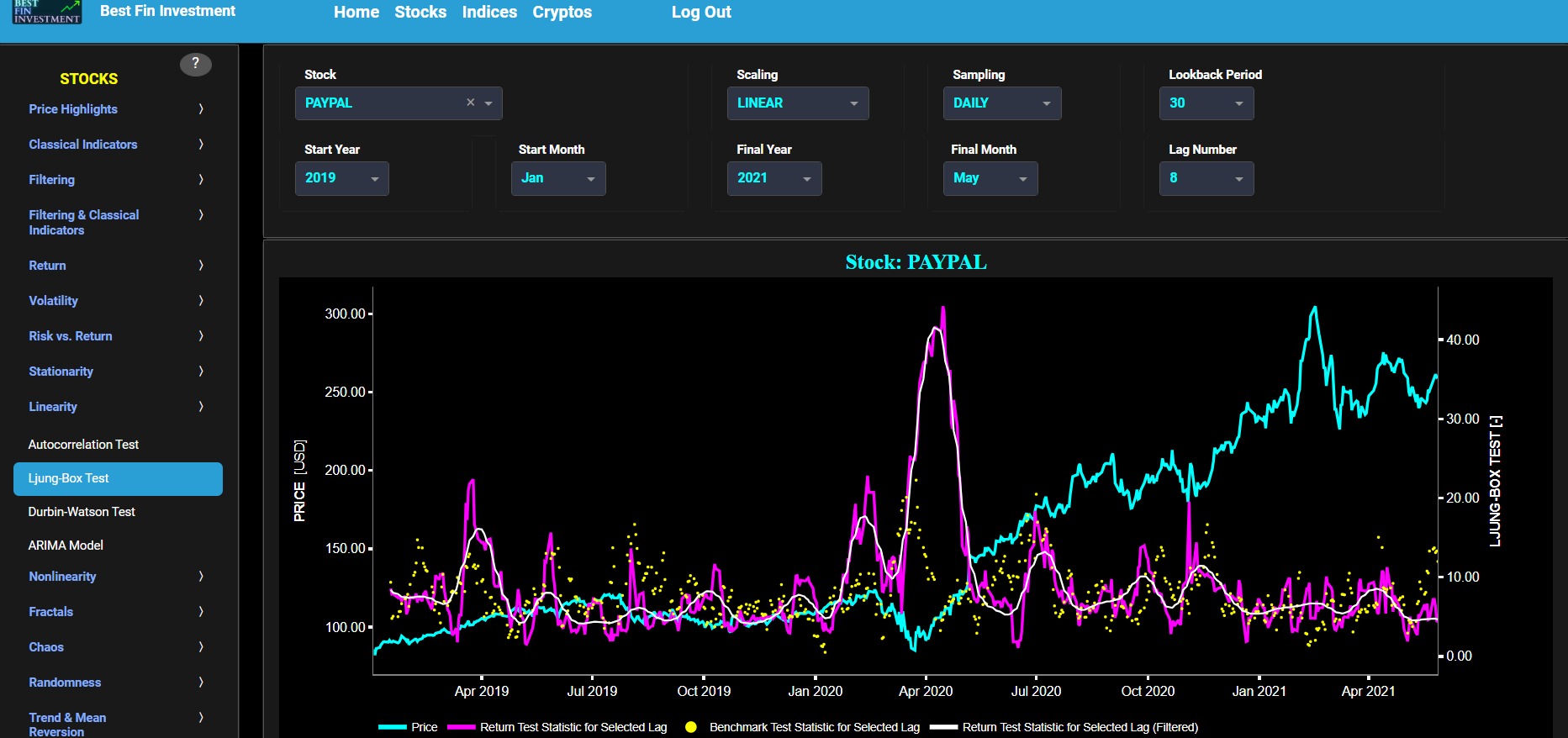
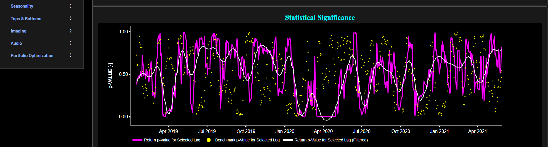
Linearity
Durbin-Watson Test
This page provides 2 graphs. The upper graph visualizes historical asset prices in cyan color using either daily, weekly, or monthly close prices. In the menu bar (located just above the graphs), you can also select specific time periods to visualize and also toggle between a linear or logarithmic price scaling on the left y-axis. Next to the cyan line, the upper graph also visualizes the statistic of the Durbin-Watson (DW) test for the asset incremental return in magenta and for a benchmark time series in yellow. This test is computed using a lookback time period that is selected in the menu bar (located just above the graphs). Now incremental return is quantified as the percentage change in the asset's price between consecutive time periods. The benchmark signal is based upon synthetically generated, normally distributed, independent and identically distributed (i.i.d.) returns. For this benchmark signal, each step is independent of the previous steps, and there is no systematic trend or pattern in the data. The yellow data points are given here for reference and comparison purposes (hence benchmarking). Next the white line represents a filtered version of the magenta line through the application of a low-pass Butterworth digital filter.
The DW statistic is a measure of autocorrelation in a time series. In this context, it quantifies whether there is any significant autocorrelation in the asset returns at lag 1. The DW null hypothesis states that there is no first-order autocorrelation (positive or negative) in the data. Now when it comes to autocorrelation it is important to recognize the following characteristics. First, linear patterns in data can result in significant autocorrelation. Hence a linear pattern is a sufficient condition for observing autocorrelation. Conversely the absence of autocorrelation guarantees the absence of linear patterns in the data. However non-linear patterns in data can also lead to autocorrelation. For instance, if a time series follows a periodic or cyclic pattern, it may exhibit autocorrelation at specific lags. Therefore, the presence of autocorrelation does not necessarily imply a linear pattern; it can also indicate non-linear dependencies (particularly when these patterns manifest themselves as spikes or oscillations in the autocorrelation). Finally the absence of significant autocorrelation does not necessarily mean that there are no non-linear patterns in the data. Non-linear patterns may not produce strong autocorrelation in these plots, especially if they are complex or irregular. Summarizing: while linear patterns will always lead to autocorrelation, non-linear patterns in the data may or may not lead to autocorrelation, depending on whether they involve systematic relationships between data points at different lags. Going back to the graph we have the following: if the DW statistic is close to 2 (i.e. around 2), it suggests no first-order autocorrelation. If the DW statistic is much less than 2 (e.g., below 1.5), it suggests positive autocorrelation meaning that there is a tendency for returns to continue in the same direction over short time intervals. If the DW statistic is much greater than 2 (e.g., above 2.5), it suggests negative autocorrelation meaning that returns have a tendency to reverse direction after a trend period.
The lower graph is in spirit similar to the upper graph except that it now computes the DW statistic for cumulative asset returns rather than incremental returns, and the yellow benchmark data reflects now a synthetically generated random walk signal. In a random walk, each step is independent of the previous steps, and there is no systematic trend or pattern in the data. The yellow random walk data points are given here for reference and comparison purposes (i.e. benchmarking).
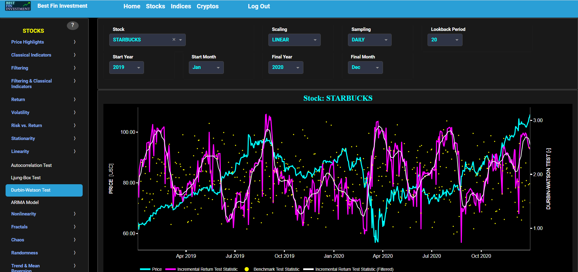
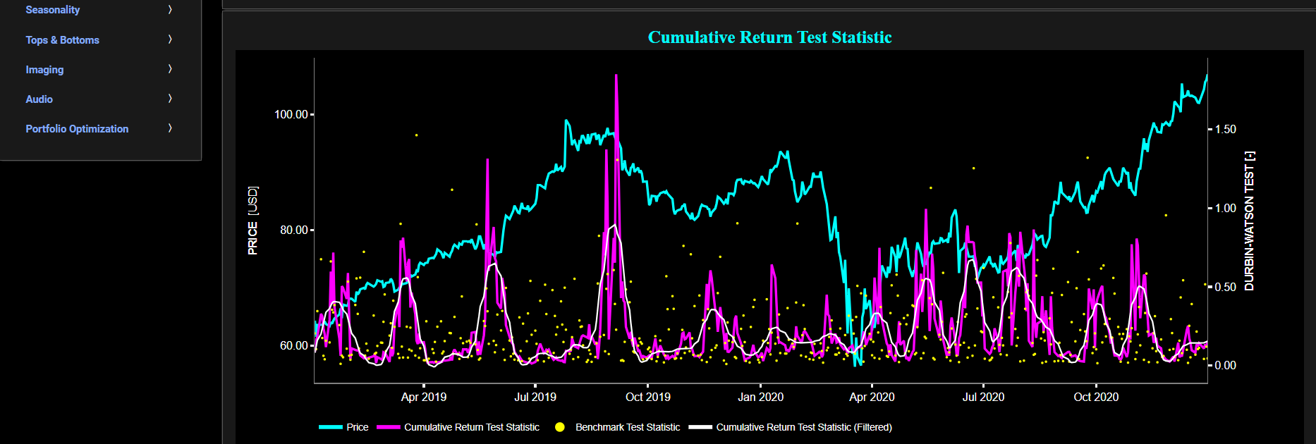
Linearity
ARIMA Model
This page provides 3 graphs. The upper graph visualizes historical asset prices in cyan color using either daily, weekly, or monthly close prices. In the menu bar (located just above the graphs), you can also select specific time periods to visualize. Next to the cyan line, the upper graph also visualizes the goodness of fit of a AutoRegressive Integrated Moving Average (ARIMA) model fitted on asset incremental returns.
Indeed ARIMA models are primarily employed to capture and model the linear dependencies and patterns within time series data, making them suitable for investigating linear behavior in asset returns. Here the upper graph uses an ARIMA(p,d,q) model which is computed using a lookback time period that is selected in the menu bar (located just above the graphs). The “p” coefficient refers to the AutoRegressive order whereas the “q”coefficient refers to the Moving Average order and both of these can be selected in the menu bar. The “d” coefficient refers to the degree of differencing and is set to zero in the upper graph.
Now the graph shows the Akaike Information Criterion (AIC) which is a measure of the goodness of fit of such an ARIMA model. The AIC balances the trade-off between model complexity and goodness of fit. In the context of ARIMA modeling, a lower (i.e. more negative) AIC value indicates a better-fitting model. Thus a lower AIC suggests a model that explains the linear patterns in asset returns more effectively. Here the graph visualizes the AIC statistic for the asset return in magenta, and for a benchmark time series in yellow. This benchmark signal is based upon synthetically generated, normally distributed, independent and identically distributed (i.i.d.) returns. For this benchmark signal, each step is independent of the previous steps, and there is no systematic trend or pattern in the data. The yellow data points are given here for reference and comparison purposes (hence benchmarking). Next the middle and lower graphs are similar in nature to the upper one, except that they plot the AIC for d=1 and d=2 respectively.
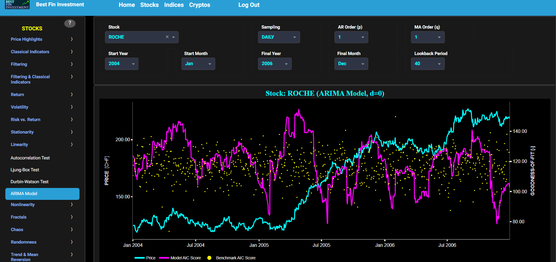
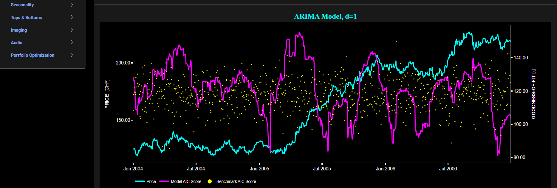
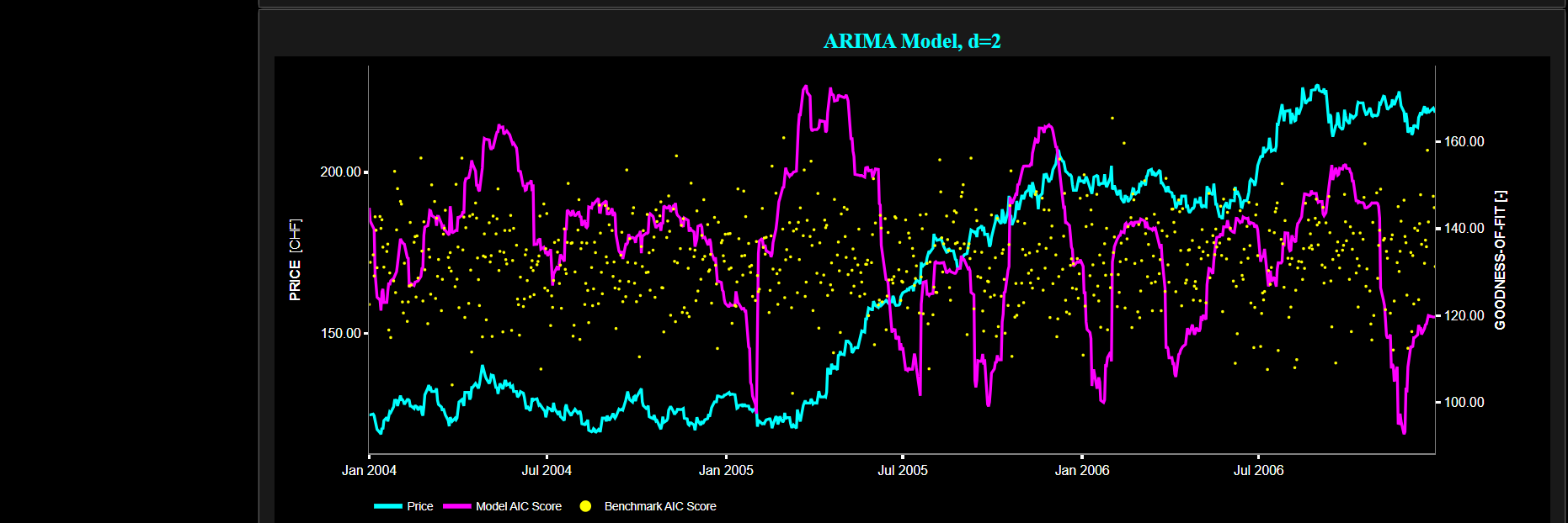
Nonlinearity
Entropy Test
This page provides 2 graphs. The upper graph visualizes historical asset prices in cyan color using either daily, weekly, or monthly close prices. In the menu bar (located just above the graphs), you can also select specific time periods to visualize and also toggle between a linear or logarithmic price scaling on the left y-axis. Next to the cyan line, the upper graph also visualizes the Binned Entropy (BE) for the asset incremental return in magenta and for a benchmark time series in yellow. The BE is computed using a lookback time period that is selected in the menu bar (located just above the graphs). Further incremental return is defined as the percentage change in the asset's price between consecutive time periods. For the benchmark signal, it is based upon synthetically generated, normally distributed, independent and identically distributed (i.i.d.) returns. For this benchmark signal, each step is independent of the previous steps, and there is no systematic trend or pattern in the data. The yellow data points are given here for reference and comparison purposes (hence benchmarking). Next the white line represents a filtered version of the magenta line through the application of a low-pass Butterworth digital filter.
The BE is a concept used in information theory and data analysis to, among others, measure a signal’s nonlinear behavior. Indeed the BE can be used to measure the degree of dispersion, disorder, or concentration of data points. It quantifies how uniformly or unevenly data is being distributed among the bins. In terms of BE interpretation we have the following: if the BE value is high, this typically indicates that the data values are more evenly distributed among the bins, hence suggesting a more “uncertain”, "random" or "nonlinear" behavior. Conversely, if the BE value is low, this generally suggests that the data values are concentrated in a few bins, which could imply more "ordered", “structured”, “regular” or "linear" behavior.
The lower graph is similar to the upper graph except that it computes the BE statistic for cumulative asset returns rather than incremental returns, and the yellow benchmark data now reflects a synthetically generated random walk signal. In a random walk, each step is independent of the previous steps, and there is no systematic trend or pattern in the data. The yellow random walk data points are given here for reference and comparison purposes (i.e. benchmarking).
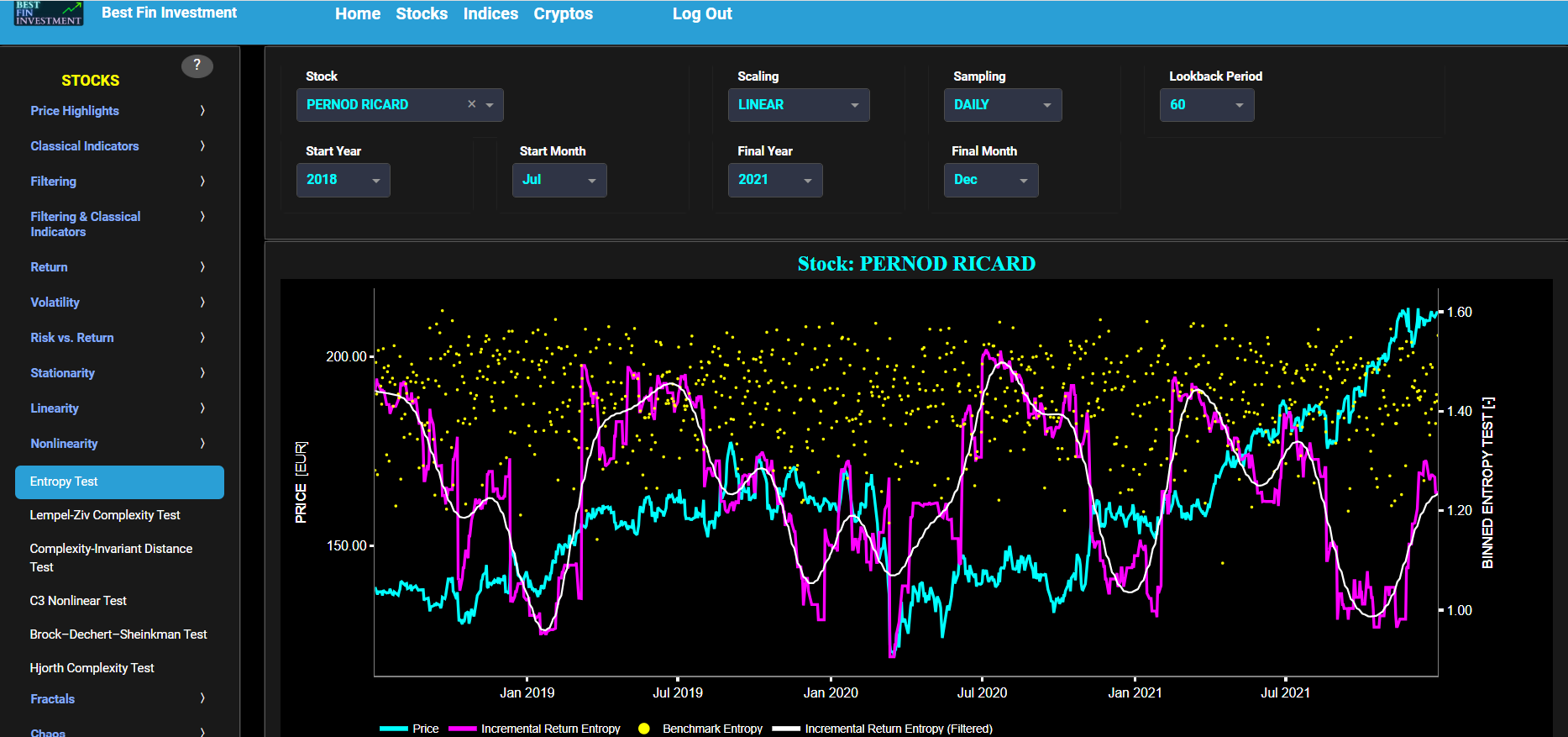
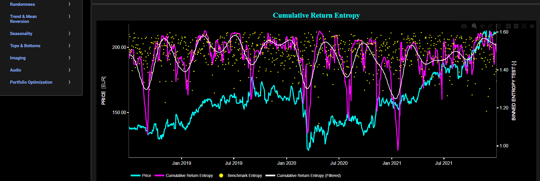
Nonlinearity
Lempel-Ziv Complexity Test
This page provides 2 graphs. The upper graph visualizes historical asset prices in cyan color using either daily, weekly, or monthly close prices. In the menu bar (located just above the graphs), you can also select specific time periods to visualize and also toggle between a linear or logarithmic price scaling on the left y-axis. Next to the cyan line, the upper graph also visualizes the Lempel-Ziv Complexity (LZC) test statistic for the asset incremental return in magenta and for a benchmark time series in yellow.
The LZC is used to analyze the complexity, regularity, or predictability of a sequence of data. Essentially the LZC provides a measure of how many different patterns exist in the sequence. Here the LZC is computed using a lookback time period that is selected in the menu bar (located just above the graphs). Further incremental return is defined as the percentage change in the asset's price between consecutive time periods. For the benchmark signal, it is based upon synthetically generated, normally distributed, independent and identically distributed (i.i.d.) returns. For this benchmark signal, each step is independent of the previous steps, and there is no systematic trend or pattern in the data. The yellow data points are given here for reference and comparison purposes (hence benchmarking). Next the white line represents a filtered version of the magenta line through the application of a low-pass Butterworth digital filter. In terms of LZC interpretation we have the following: high complexity suggests that the data has many unique patterns, which may indicate nonlinearity, irregularity, or unpredictability. Conversely, low complexity suggests that the data has fewer unique patterns, potentially indicating a more ordered or predictable behavior.
The lower graph is similar to the upper graph except that it computes the LZC statistic for cumulative asset returns rather than incremental returns, and the yellow benchmark data now reflects a synthetically generated random walk signal. In a random walk, each step is independent of the previous steps, and there is no systematic trend or pattern in the data. The yellow random walk data points are given here for reference and comparison purposes (i.e. benchmarking).
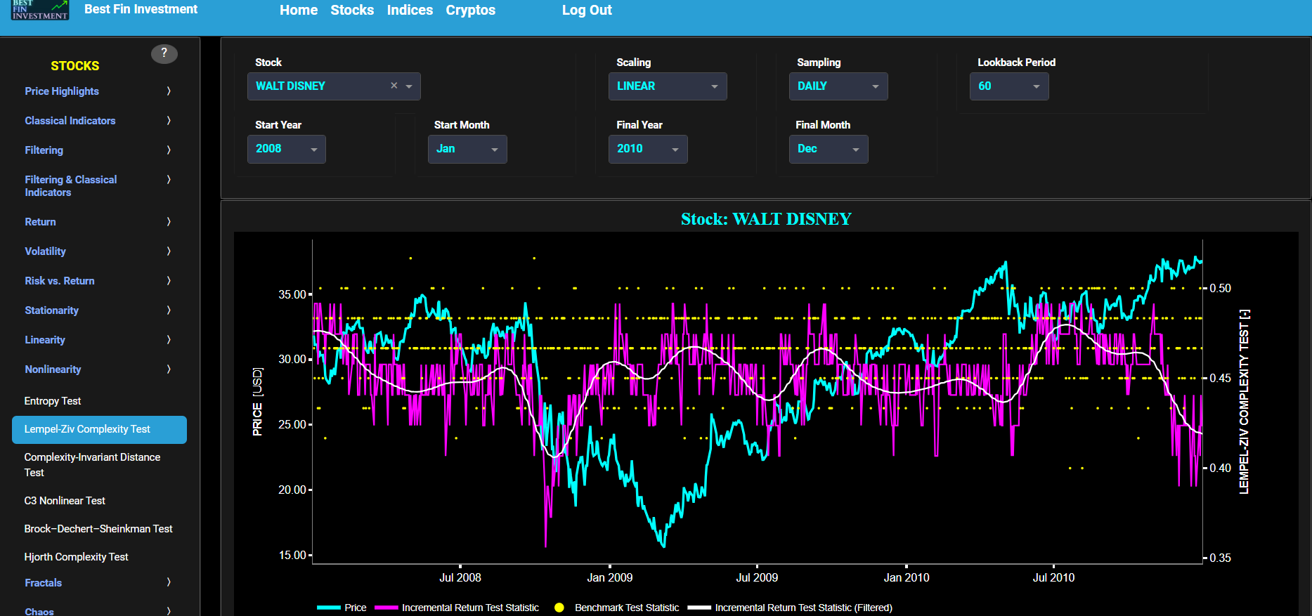
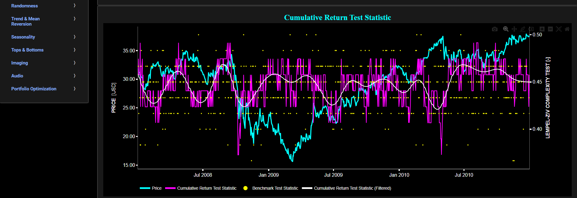
Nonlinearity
Complexity-Invariant Distance Test
This page provides 2 graphs. The upper graph visualizes historical asset prices in cyan color using either daily, weekly, or monthly close prices. In the menu bar (located just above the graphs), you can also select specific time periods to visualize and also toggle between a linear or logarithmic price scaling on the left y-axis. Next to the cyan line, the upper graph also visualizes the Complexity-Invariant Distance (CID) test statistic for the asset incremental return in magenta and for a benchmark time series in yellow.
The CID is a measure of the complexity or irregularity of a time series sequence and is used to assess the nonlinear behavior of asset returns, and further detect irregular patterns or complex dynamics in financial time series. Here the CID is computed using a lookback time period that is selected in the menu bar (located just above the graphs). Further incremental return is defined as the percentage change in the asset's price between consecutive time periods. For the benchmark signal, it is based upon synthetically generated, normally distributed, independent and identically distributed (i.i.d.) returns. For this benchmark signal, each step is independent of the previous steps, and there is no systematic trend or pattern in the data. The yellow data points are given here for reference and comparison purposes (hence benchmarking). Next the white line represents a filtered version of the magenta line through the application of a low-pass Butterworth digital filter. In terms of CID interpretation we have the following: if the CID is high, it suggests that the sequence exhibits more complexity, nonlinearity or irregularity. If the CID is low, it suggests that the sequence is more regular or linear. A CID value of 0.0 typically indicates that the input sequence was constant or unchanging, which implies no complexity. A significant change in CID over time may suggest changes in the underlying dynamics of the data, which could be associated with nonlinear behavior.
The lower graph is similar to the upper graph except that it computes the CID statistic for cumulative asset returns rather than incremental returns, and the yellow benchmark data now reflects a synthetically generated random walk signal. In a random walk, each step is independent of the previous steps, and there is no systematic trend or pattern in the data. The yellow random walk data points are given here for reference and comparison purposes (i.e. benchmarking).
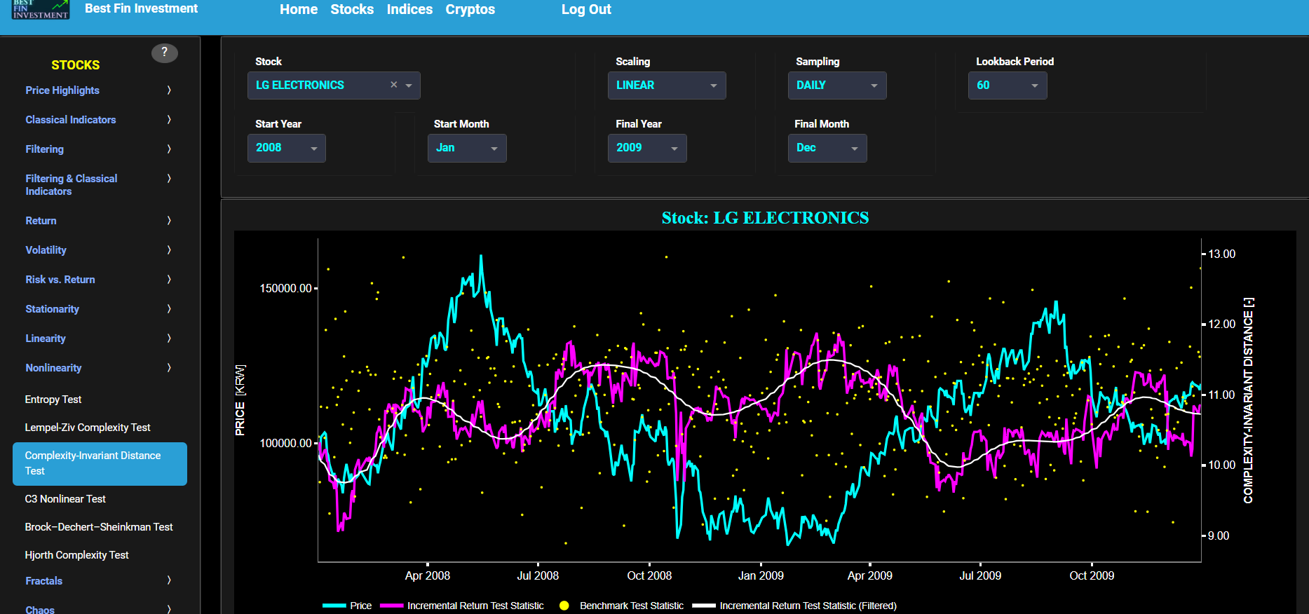
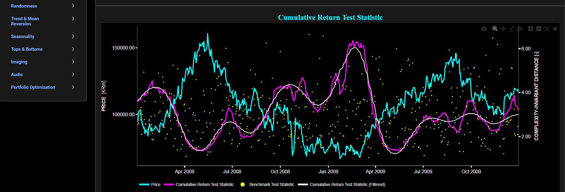
Nonlinearity
C3 Nonlinear Test
This page provides 2 graphs. The upper graph visualizes historical asset prices in cyan color using either daily, weekly, or monthly close prices. In the menu bar (located just above the graphs), you can also select specific time periods to visualize and also toggle between a linear or logarithmic price scaling on the left y-axis. Next to the cyan line, the upper graph also visualizes the C3 test statistic for the asset incremental return in magenta and for a benchmark time series in yellow.
The C3 is used to detect nonlinear dependencies or cubic nonlinear relationships within a time series. The C3 statistic is more commonly used in fields such as signal processing and control systems. Here the C3 is computed using a lookback time period that is selected in the menu bar (located just above the graphs). You can also specify a lag value in the menu bar (located just above the graphs). This lag value is applied to the input time series data to create shifted or delayed versions of the sequence. By comparing these shifted sequences with the original data, the C3 metric evaluates the degree of nonlinearity in the data. Now incremental return is defined as the percentage change in the asset's price between consecutive time periods. For the benchmark signal, it is based upon synthetically generated, normally distributed, independent and identically distributed (i.i.d.) returns. For this benchmark signal, each step is independent of the previous steps, and there is no systematic trend or pattern in the data. The yellow data points are given here for reference and comparison purposes (hence benchmarking). Next the white line represents a filtered version of the magenta line through the application of a low-pass Butterworth digital filter. In terms of C3 interpretation we have the following: if the C3 statistic is close to zero, it suggests a weak or negligible cubic nonlinear relationship between past and future values of the time series. In this case, the time series may exhibit more linear behavior. If the C3 statistic is significantly different from zero (either positive or negative), it indicates the presence of a cubic nonlinear relationship within the time series.
The lower graph is similar to the upper graph except that it computes the C3 statistic for cumulative asset returns rather than incremental returns, and the yellow benchmark data now reflects a synthetically generated random walk signal. In a random walk, each step is independent of the previous steps, and there is no systematic trend or pattern in the data. The yellow random walk data points are given here for reference and comparison purposes (i.e. benchmarking).
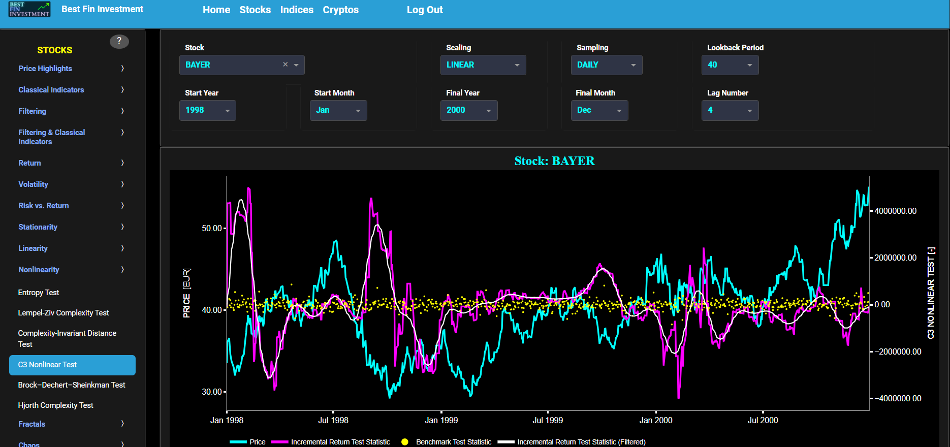
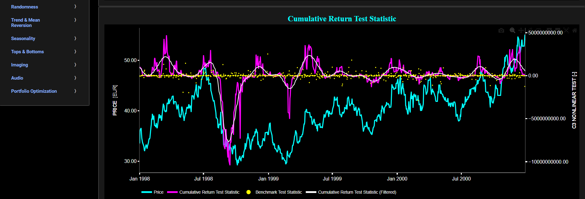
Nonlinearity
Brock–Dechert–Sheinkman Test
This page provides 2 graphs. The upper graph visualizes historical asset prices in cyan color using either daily, weekly, or monthly close prices. In the menu bar (located just above the graphs), you can also select specific time periods to visualize and also toggle between a linear or logarithmic price scaling on the left y-axis. Next to the cyan line, the upper graph also visualizes the Brock–Dechert–Sheinkman (BDS) test statistic for the asset incremental return in magenta and for a benchmark time series in yellow.
The BDS uses Machine Learning (ML) to detect nonlinear dependencies or nonlinear patterns within a time series. In our case the BDS is used to measure the nonlinear behavior of incremental return patterns, using a lookback time period that is selected in the menu bar (located just above the graphs). Further incremental return is defined as the percentage change in the asset's price between consecutive time periods. For the benchmark signal, it is based upon synthetically generated, normally distributed, independent and identically distributed (i.i.d.) returns. For this benchmark signal, each step is independent of the previous steps, and there is no systematic trend or pattern in the data. The yellow data points are given here for reference and comparison purposes (hence benchmarking). In terms of BDS interpretation we have the following: if the BDS statistic is significantly different from zero, it suggests the presence of nonlinear dependencies or non-random behavior in the time series. Further the test sensitivity can also be adjusted in the menu bar (located just above the graphs).
The lower graph is similar to the upper graph except that it computes the BDS statistic for cumulative asset returns rather than incremental returns, and the yellow benchmark data now reflects a synthetically generated random walk signal. In a random walk, each step is independent of the previous steps, and there is no systematic trend or pattern in the data. The yellow random walk data points are given here for reference and comparison purposes (i.e. benchmarking).
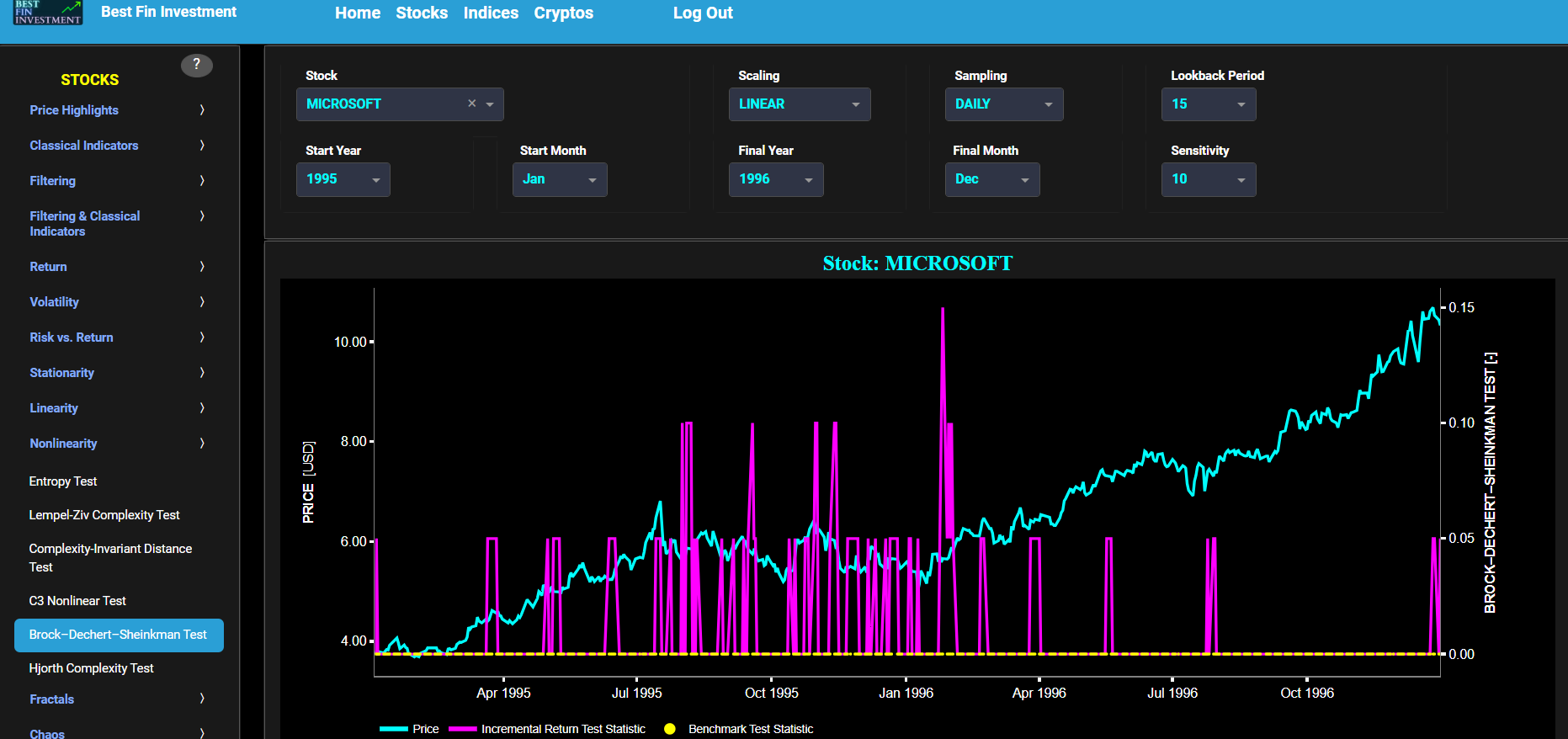
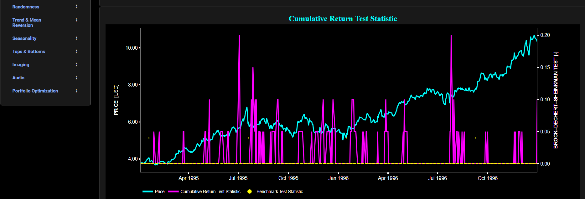
Nonlinearity
Hjorth Complexity Test
This page provides 2 graphs. The upper graph visualizes historical asset prices in cyan color using either daily, weekly, or monthly close prices. In the menu bar (located just above the graphs), you can also select specific time periods to visualize and also toggle between a linear or logarithmic price scaling on the left y-axis. Next to the cyan line, the upper graph also visualizes the Hjorth Complexity (HC) test statistic for the asset incremental return in magenta and for a benchmark time series in yellow.
The HC is a metric based upon the so-called Hjorth Mobility. These metrics provide insights into the nonlinear characteristics of a time series by measuring its complexity or irregularity. Named after the Danish neuroscientist Bjorn H. Hjorth, these signal metrics were originally introduced and widely used in the field of neurophysiology and electroencephalography (EEG), to characterize brain wave patterns and assess the complexity of neural signals (e.g. detection of abnormalities or changes in neurological conditions). Over time these metrics have found applications in other fields, beyond neuroscience, such as in finance and time series analysis. Here the HC is computed using a lookback time period that is selected in the menu bar (located just above the graphs). Further incremental return is defined as the percentage change in the asset's price between consecutive time periods. For the benchmark signal, it is based upon synthetically generated, normally distributed, independent and identically distributed (i.i.d.) returns. For this benchmark signal, each step is independent of the previous steps, and there is no systematic trend or pattern in the data. The yellow data points are given here for reference and comparison purposes (hence benchmarking). Next the white line represents a filtered version of the magenta line through the application of a low-pass Butterworth digital filter. In terms of HC interpretation we have the following: high HC values may suggest that the time series exhibits complex and irregular patterns, which could basically be indicative of nonlinear behavior.
The lower graph is similar to the upper graph except that it computes the HC statistic for cumulative asset returns rather than incremental returns, and the yellow benchmark data now reflects a synthetically generated random walk signal. In a random walk, each step is independent of the previous steps, and there is no systematic trend or pattern in the data. The yellow random walk data points are given here for reference and comparison purposes (i.e. benchmarking).
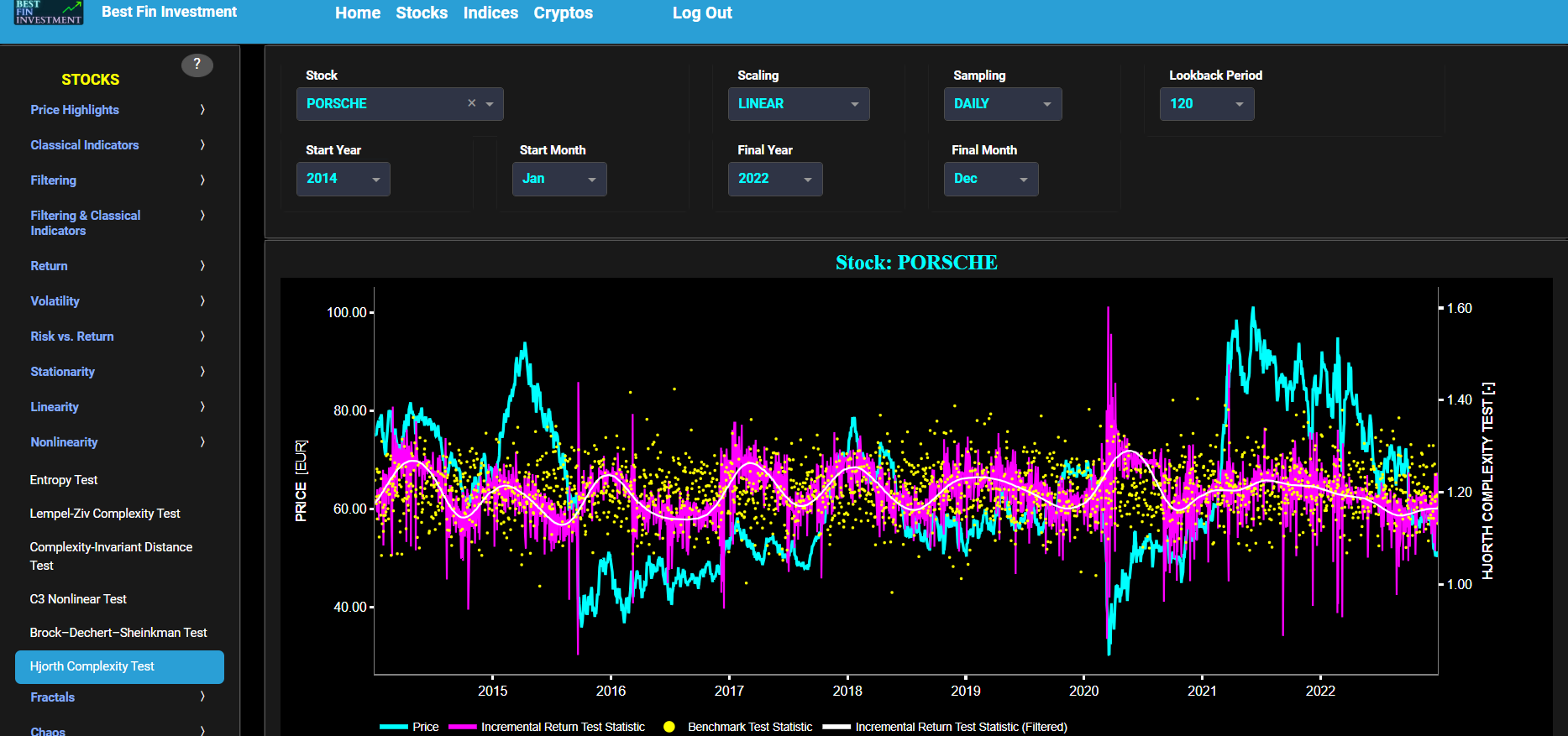
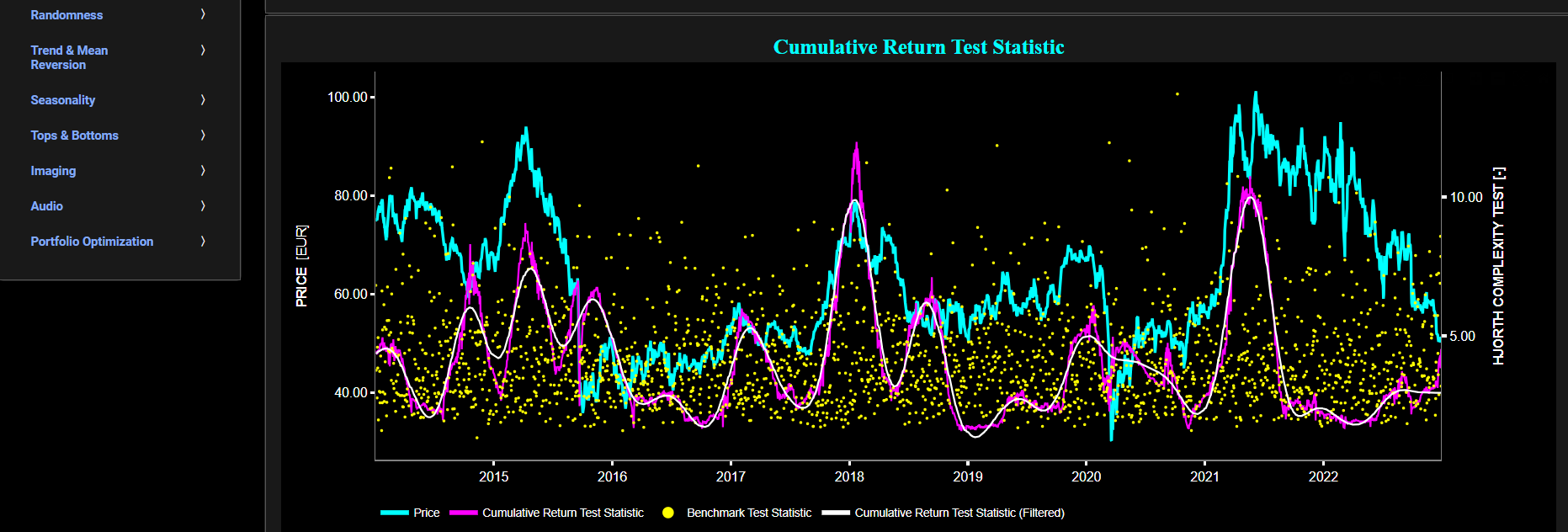
Fractals
Petrosian Fractal Dimension
This page provides 2 graphs. The upper graph visualizes historical asset prices in cyan color using either daily, weekly, or monthly close prices. In the menu bar (located just above the graphs), you can also select specific time periods to visualize and also toggle between a linear or logarithmic price scaling on the left y-axis. Next to the cyan line, the upper graph also visualizes the Petrosian Fractal Dimension (PFD) test statistic for the asset incremental return in magenta and for a benchmark time series in yellow.
The PFD is a measure of signal irregularity or fractal-like behavior (also known as self-similarity) in a time series. The PFD was originally developed and widely used in the field of biomedical signal analysis, particularly in electroencephalography (EEG) signal analysis. In EEG analysis, the PFD can provide insights into the complexity of brain wave patterns, helping researchers understand neural activity and detect abnormalities. The PFD is particularly used when the focus is on abrupt changes, spikes, or irregularities in the data, as the PFD is sensitive to rapid sign changes and is hence suitable for capturing non-smooth patterns. Now returning to finance, when we say that a price series exhibits more fractal-like or self-similar behavior, it means that the price or asset return movements within that series display patterns or structures at multiple scales, and these patterns tend to repeat themselves when you zoom in or out on the data (e.g. the same patterns may be identified over a few minutes, hours, days, and weeks in a financial time series). This concept is closely related to the idea of fractals, which are mathematical objects characterized by self-similarity. Here the PFD is computed using a lookback time period that is selected in the menu bar (located just above the graphs). Further incremental return is defined as the percentage change in the asset's price between consecutive time periods. For the benchmark signal, it is based upon synthetically generated, normally distributed, independent and identically distributed (i.i.d.) returns. For this benchmark signal, each step is independent of the previous steps, and there is no systematic trend or pattern in the data. The yellow data points are given here for reference and comparison purposes (hence benchmarking). Next the white line represents a filtered version of the magenta line through the application of a low-pass Butterworth digital filter. In terms of PFD interpretation we have the following: a higher PFD value typically indicates a higher degree of irregularity, complexity, or fractal-like behavior in the time series. A lower PFD suggests smoother, less irregular behavior in the data.
The lower graph is similar to the upper graph except that it computes the PFD statistic for cumulative asset returns rather than incremental returns, and the yellow benchmark data now reflects a synthetically generated random walk signal. In a random walk, each step is independent of the previous steps, and there is no systematic trend or pattern in the data. The yellow random walk data points are given here for reference and comparison purposes (i.e. benchmarking).
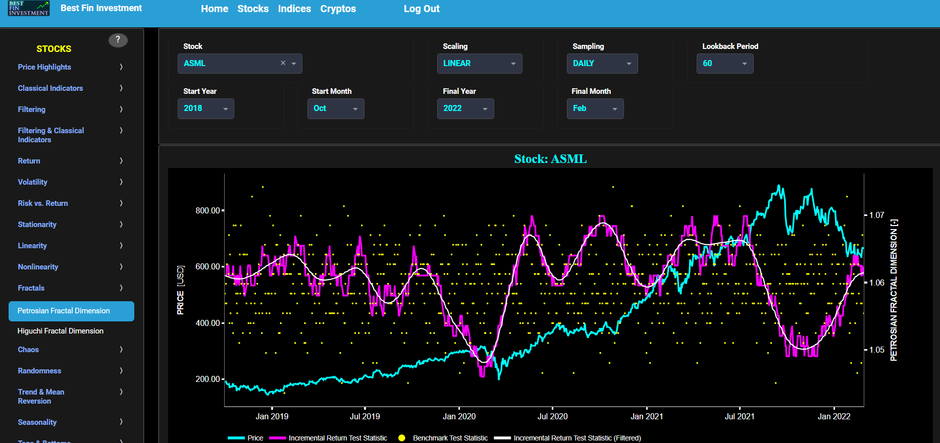
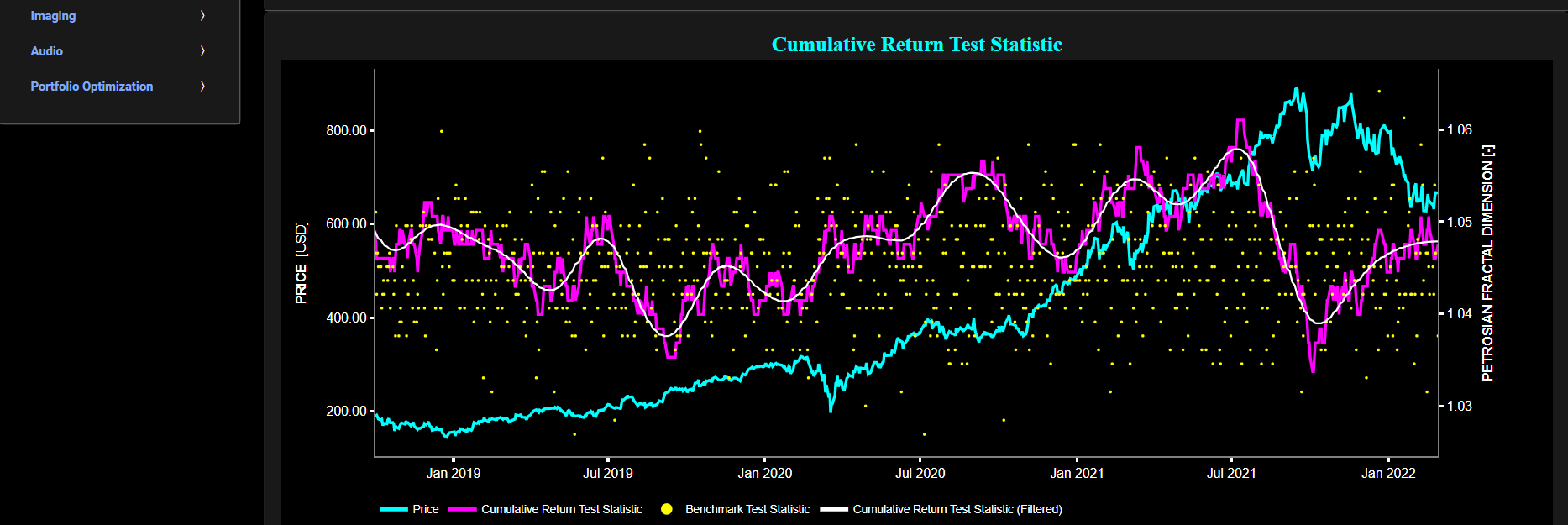
Fractals
Higuchi Fractal Dimension
This page provides 2 graphs. The upper graph visualizes historical asset prices in cyan color using either daily, weekly, or monthly close prices. In the menu bar (located just above the graphs), you can also select specific time periods to visualize and also toggle between a linear or logarithmic price scaling on the left y-axis. Next to the cyan line, the upper graph also visualizes the Higuchi Fractal Dimension (HFD) test statistic for the asset incremental return in magenta and for a benchmark time series in yellow.
The HFD is a measure of signal irregularity or fractal-like behavior (also known as self-similarity) in a time series. The HFD was originally developed by Dr. Tomoyuki Higuchi, a Japanese researcher who made contributions to the field of fractal analysis and signal processing. The HFD was used in various fields, including biomedical signal analysis such as in electroencephalography (EEG) signal analysis. In EEG analysis, the HFD can provide insights into the complexity of brain wave patterns, helping researchers understand neural activity and detect abnormalities. The HFD is particularly used to assess local variations and fine-scale self-similarity in data. It may be more suitable for capturing subtle fractal-like behavior within smaller segments of a time series. Now returning to finance, when we say that a price series exhibits more fractal-like or self-similar behavior, it means that the price or asset return movements within that series display patterns or structures at multiple scales, and these patterns tend to repeat themselves when you zoom in or out on the data (e.g. the same patterns may be identified over a few minutes, hours, days, and weeks in a financial time series). This concept is closely related to the idea of fractals, which are mathematical objects characterized by self-similarity. Here the HFD is computed using a lookback time period that is selected in the menu bar (located just above the graphs). Further incremental return is defined as the percentage change in the asset's price between consecutive time periods. For the benchmark signal, it is based upon synthetically generated, normally distributed, independent and identically distributed (i.i.d.) returns. For this benchmark signal, each step is independent of the previous steps, and there is no systematic trend or pattern in the data. The yellow data points are given here for reference and comparison purposes (hence benchmarking). Next the white line represents a filtered version of the magenta line through the application of a low-pass Butterworth digital filter. In terms of HFD interpretation we have the following: a higher HFD value typically indicates a higher degree of irregularity, complexity, or fractal-like behavior in the time series. A lower HFD suggests smoother, less irregular behavior in the data.
The lower graph is similar to the upper graph except that it computes the HFD statistic for cumulative asset returns rather than incremental returns, and the yellow benchmark data now reflects a synthetically generated random walk signal. In a random walk, each step is independent of the previous steps, and there is no systematic trend or pattern in the data. The yellow random walk data points are given here for reference and comparison purposes (i.e. benchmarking).
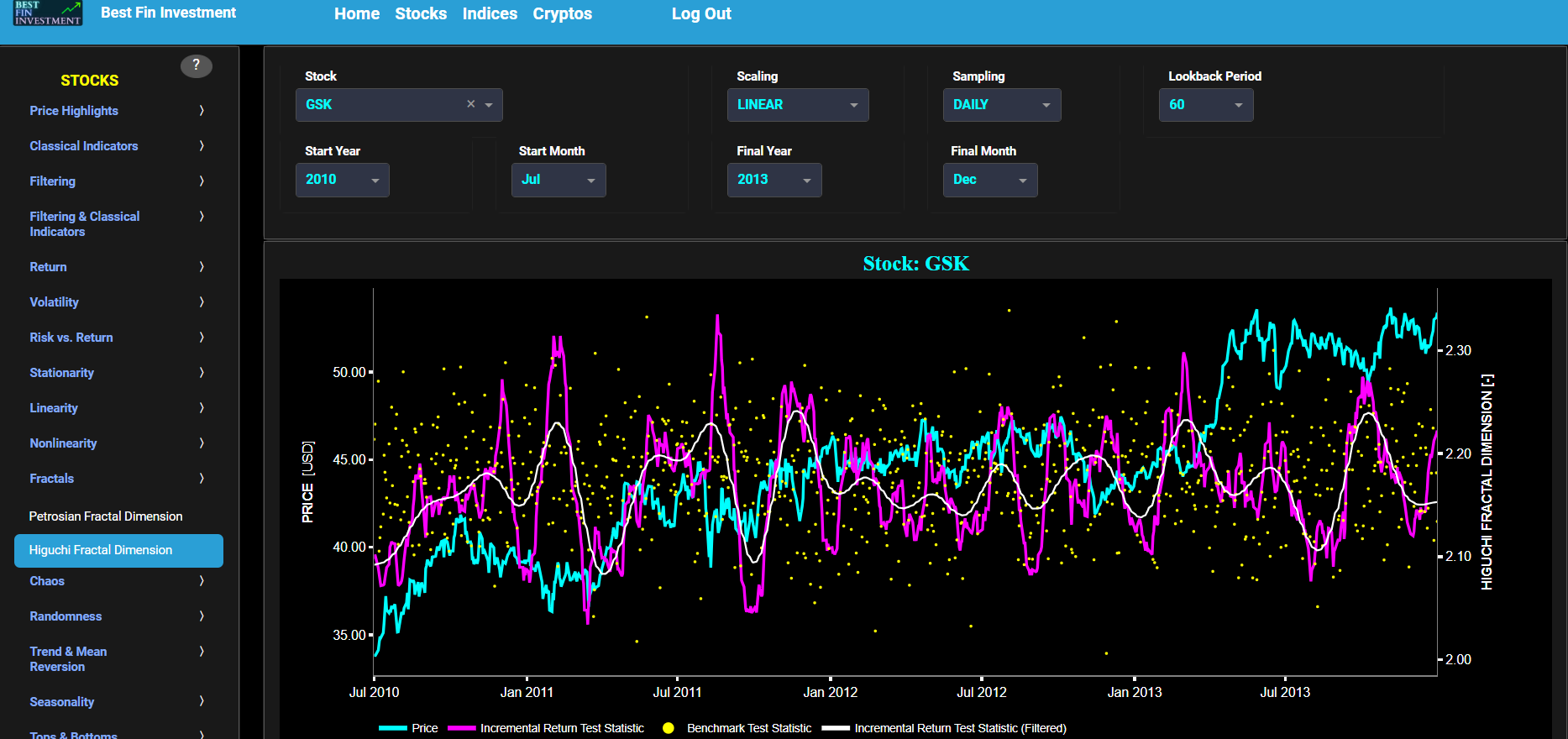
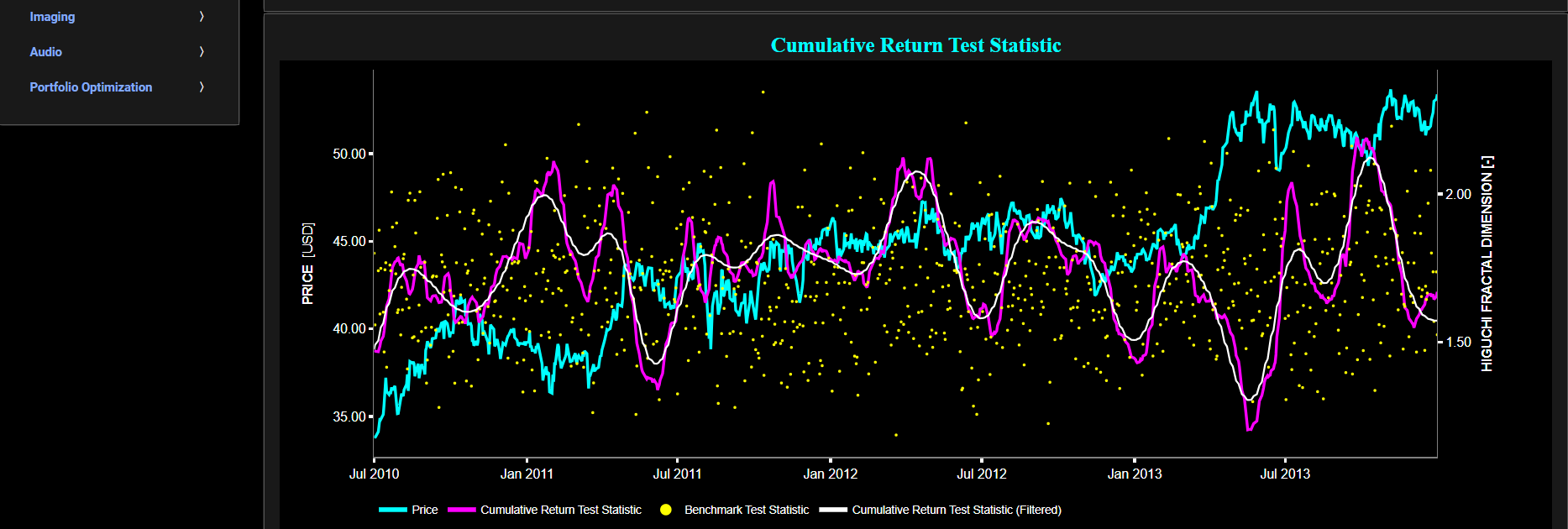
Chaos
Lyapunov Exponent
This page provides 2 graphs. The upper graph visualizes historical asset prices in cyan color using either daily, weekly, or monthly close prices. In the menu bar (located just above the graphs), you can also select specific time periods to visualize and also toggle between a linear or logarithmic price scaling on the left y-axis. Next to the cyan line, the upper graph also visualizes the Lyapunov Exponent (LE) statistic for the asset price in magenta and for a synthetically generated random walk in yellow color. In a random walk, each step is independent of the previous steps, and there is no systematic trend or pattern in the data. The yellow random walk data points are given here for reference and comparison purposes (i.e. benchmarking).
The LE is a measure of the rate of divergence of nearby trajectories in a chaotic dynamical system. The LE is commonly used in the field of nonlinear dynamics, nonlinear control theory, and chaos theory to quantify the stability and chaotic behavior of dynamical systems. The LE was first introduced by the Russian mathematician Aleksandr Lyapunov in the late 19th century as part of his work on the stability of dynamical systems. It has since found applications in the study of chaos and complex systems in various scientific disciplines. Here the LE is computed using a lookback time period that is selected in the menu bar (located just above the graphs). Next the white line represents a filtered version of the magenta line through the application of a low-pass Butterworth digital filter. In terms of LE interpretation we have the following: if the LE is consistently negative, it indicates that nearby trajectories in the system are converging, which implies stability. This is often the case for well-behaved systems with predictable dynamics. Next a LE equal to zero suggests that nearby trajectories neither converge nor diverge significantly over time. This can occur in systems with periodic or quasi-periodic behavior. Lastly, a positive LE indicates chaotic behavior. The larger the positive value, the faster nearby trajectories diverge, and the more unpredictable and chaotic the system's behavior becomes, which suggests that the time series movements may be hard to predict. Note that the LE test sensitivity can also be adjusted in the menu bar (located just above the graphs).
Regarding the lower graph, this latter visualizes the asset price in cyan color, and the LE statistic for the asset incremental return in magenta together with the LE statistic for a benchmark signal in yellow. Incremental return is defined as the percentage change in the asset's price between consecutive time periods, whereas the benchmark signal is based upon synthetically generated, normally distributed, independent and identically distributed (i.i.d.) returns. For this benchmark signal, each step is independent of the previous steps, and there is no systematic trend or pattern in the data.
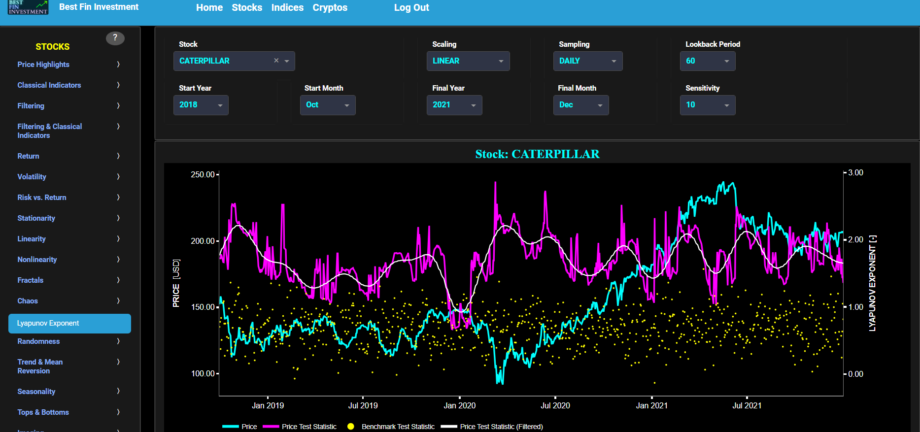
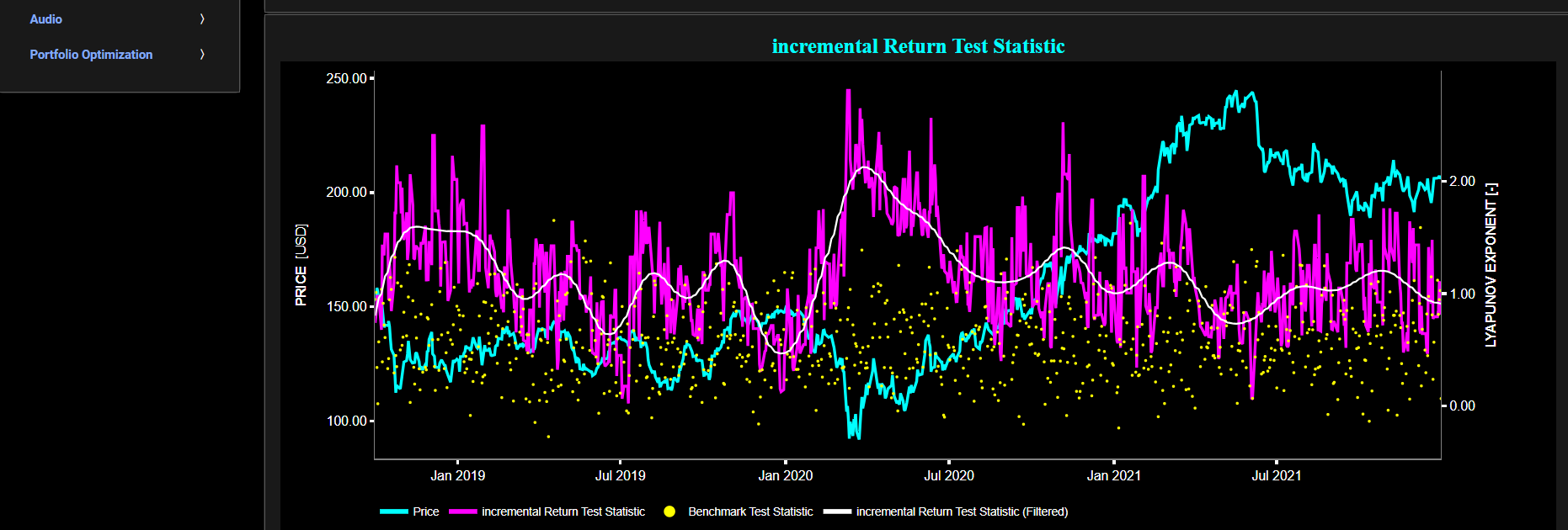
Randomness
Variance Ratio Test
This page provides 2 graphs. The upper graph visualizes historical asset prices in cyan color using either daily, weekly, or monthly close prices. In the menu bar (located just above the graphs), you can also select specific time periods to visualize and also toggle between a linear or logarithmic price scaling on the left y-axis. Next to the cyan line, the upper graph also visualizes the statistic of the Variance Ratio (VR) test for the asset price in magenta, and for a synthetically generated random walk in yellow color. In a random walk, each step is independent of the previous steps, and there is no systematic trend or pattern in the data. The yellow random walk data points are given here for reference and comparison purposes (i.e. benchmarking).
The VR test is a statistical test that was introduced by Andrew W. Lo & A. Craig MacKinlay, 1987, "Stock Market Prices Do Not Follow Random Walks: Evidence From a Simple Specification Test," NBER Working Papers 2168, National Bureau of Economic Research, Inc. This test is typically applied to financial time series data to assess whether the data follows a random walk, which is a hypothesis often associated with efficient markets. Essentially the test checks for the presence of serial correlation or autocorrelation in the time series. The underlying assumption is that if a time series follows a random walk, the variance of returns over longer time intervals should be proportional to the length of those intervals. Deviations from this proportional relationship suggest the presence of serial correlation. The null hypothesis of a VR is that the process is a random walk, possibly plus drift. Rejection of the null with a positive test statistic indicates the presence of positive serial correlation in the time series. This test is computed using a lookback time period that is selected in the menu bar (located just above the graphs). Further you can also select the lag number, i.e. the number of periods to be used in the multi-period variance test. Next the white line represents a filtered version of the magenta line through the application of a low-pass Butterworth digital filter. While users may intuitively expect the test to return a VR value close to 1 when the series is random, the test itself returns a standardized test statistic, not the raw VR value. In terms of result interpretation we have the following: if the VR test is close to 0, it suggests that the series follows a random walk (efficient market hypothesis, meaning the raw VR value is close to 1). A VR significantly different from 0 may indicate deviations from a random walk, implying potential predictability or serial correlation in the data. A significantly negative test statistic suggests mean reversion (prices tend to reverse), while a significantly positive one points to momentum (prices tend to continue in the same direction).
Next the lower graph visualizes the statistical significance (p-value) of the VR test for the asset price in magenta, and for the benchmark signal in yellow. The p-value associated with the VR statistic indicates the probability of obtaining a test statistic as extreme as the one observed if the null hypothesis were true. A small p-value (typically less than a significance level, e.g., 0.05) suggests evidence against the random walk hypothesis (i.e. against the null hypothesis), hence indicating some form of predictability or serial correlation.
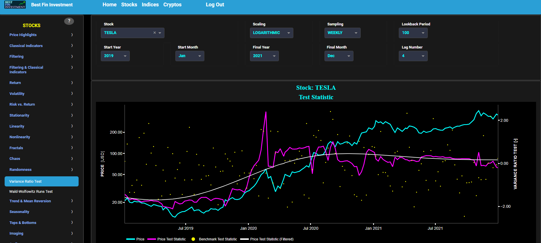
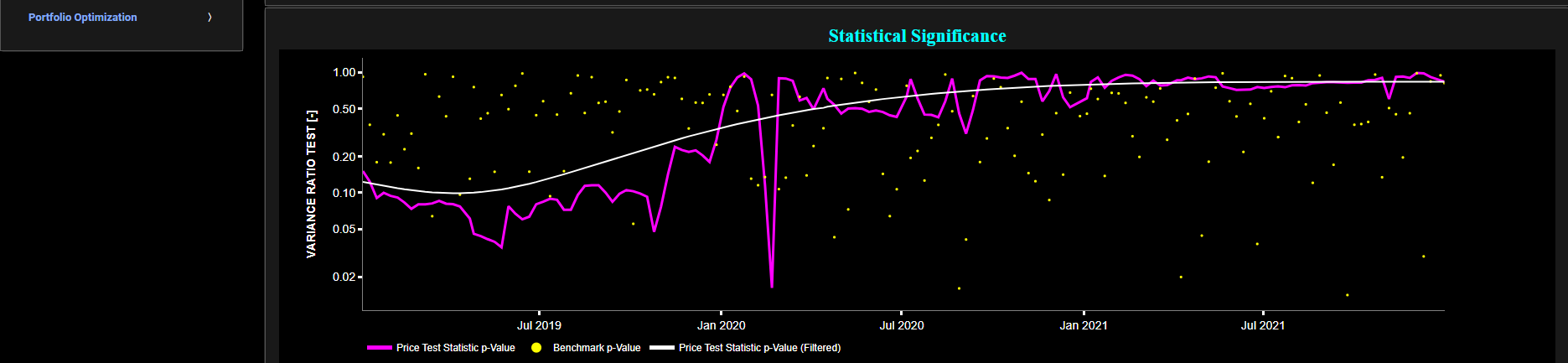
Randomness
Wald-Wolfowitz Runs Test
This page provides 2 graphs. The upper graph visualizes historical asset prices in cyan color using either daily, weekly, or monthly close prices. In the menu bar (located just above the graphs), you can also select specific time periods to visualize and also toggle between a linear or logarithmic price scaling on the left y-axis. Next to the cyan line, the upper graph also visualizes the statistic of the Wald-Wolfowitz Runs (WWR) test for the asset incremental return in magenta and for a benchmark time series in yellow. Incremental return is defined as the percentage change in the asset's price between consecutive time periods. For the benchmark signal, it is based upon synthetically generated, normally distributed, independent and identically distributed (i.i.d.) returns. For this benchmark signal, each step is independent of the previous steps, and there is no systematic trend or pattern in the data. The yellow data points are given here for reference and comparison purposes (hence benchmarking).
The WWR test can help assess whether there are non-random patterns or structures in the sequence of asset returns. Specifically, it checks whether there is evidence of serial correlation or runs of similar behavior in the data. The null hypothesis for the WWR test is that the data is a random sequence with no underlying pattern in the runs. The WWR test is computed using a lookback time period that is selected in the menu bar (located just above the graphs). Next the white line represents a filtered version of the magenta line through the application of a low-pass Butterworth digital filter. In terms of result interpretation we have the following: if the test statistic is far from zero, it may indicate a significant departure from randomness. A positive test statistic indicates that the signs (positive/negative) of the returns alternate more frequently, suggesting negative serial correlation or mean-reverting behavior. Conversely, a negative test statistic indicates longer clusters of the same sign (e.g., several consecutive positive or negative returns), suggesting positive serial correlation or momentum/trending behavior.
Next the lower graph visualizes the statistical significance (p-value) of the WWR test for the asset return in magenta, and for the benchmark signal in yellow. The p-value associated with the WWR statistic indicates the probability of obtaining a test statistic as extreme as the one observed if the null hypothesis were true. A small p-value (typically less than a significance level, e.g., 0.05) suggests evidence against the random walk hypothesis (i.e. against the null hypothesis), hence indicating the presence of non-random patterns in the data.
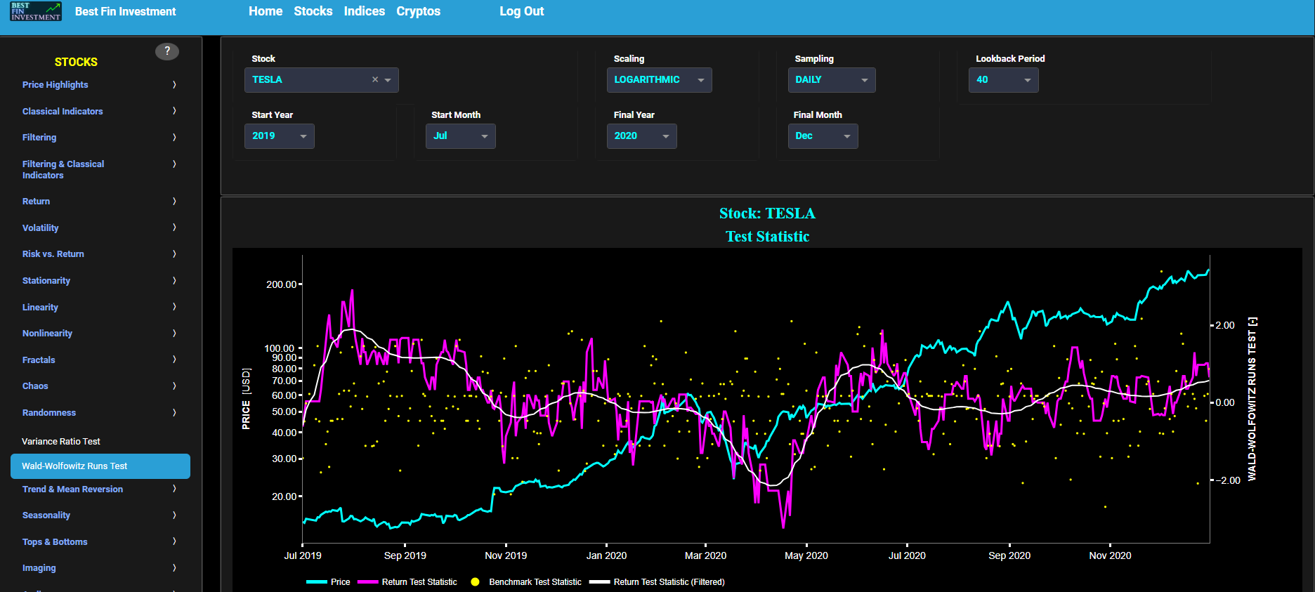
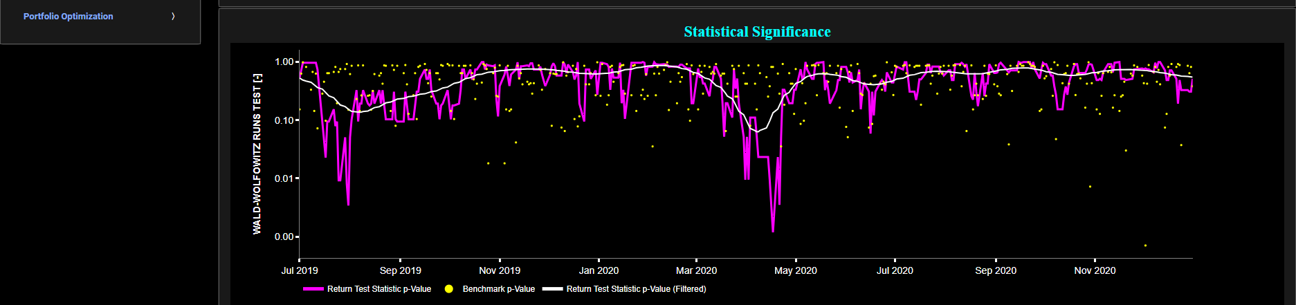
Trend & Mean Reversion
Simple Moving Average
This page provides 2 graphs. The upper graph visualizes historical asset prices in cyan color using either daily, weekly, or monthly close prices. In the menu bar (located just above the graphs), you can also select specific time periods to visualize and also toggle between a linear or logarithmic price scaling on the left y-axis. In addition the upper graph allows you to superimpose several Simple Moving Average (SMA) lines. Next to the asset price line in cyan color, the graph also visualizes an additional user-defined SMA in magenta color. The lookback time period for this latter line can be selected in the menu bar (located just above the graphs). The lower graph shows in magenta color the percentage Rate Of Change (ROC) of the user-defined SMA line, between consecutive time periods. Next a filtered version of this magenta ROC line is computed through the application of a low-pass Butterworth digital filter. Here all positive values (above the zero horizontal white line) of the filtered ROC are shown in green color dots whereas all negative values (below the zero horizontal white line) of the filtered ROC are shown in red color dots. The information presented in both graphs can be combined to identify potential price trend patterns.
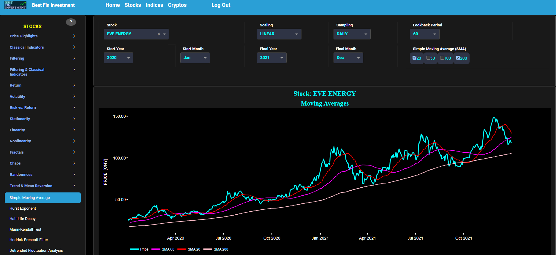
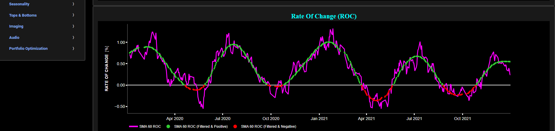
Trend & Mean Reversion
Exponential Moving Average
This page provides 2 graphs. The upper graph visualizes historical asset prices in cyan color using either daily, weekly, or monthly close prices. In the menu bar (located just above the graphs), you can also select specific time periods to visualize and also toggle between a linear or logarithmic price scaling on the left y-axis. In addition the upper graph allows you to superimpose several Simple Moving Average (SMA) lines. Next to the asset price line in cyan color, the graph also visualizes an additional user-defined Exponential Moving Average (EMA) in magenta color. The EMA lookback time period (which is driving the decay rate) can be selected in the menu bar (located just above the graphs).
Indeed EMA’s represent useful metrics towards the identification of price trend patterns, see for example the results presented in the paper by: Y. Lemperiere, C. Deremble, P. Seager, M. Potters, J.-P. Bouchaud, "Two centuries of trend following", J. Invest. Strateg., 3(3), pp. 41-61, 2014. Now the lower graph shows in magenta color the percentage Rate Of Change (ROC) of the user-defined EMA line, between consecutive time periods. Next a filtered version of this magenta ROC line is computed through the application of a low-pass Butterworth digital filter. Here all positive values (above the zero horizontal white line) of the filtered ROC are shown in green color dots whereas all negative values (below the zero horizontal white line) of the filtered ROC are shown in red color dots. The information presented in both graphs can be combined to identify potential price trend patterns.
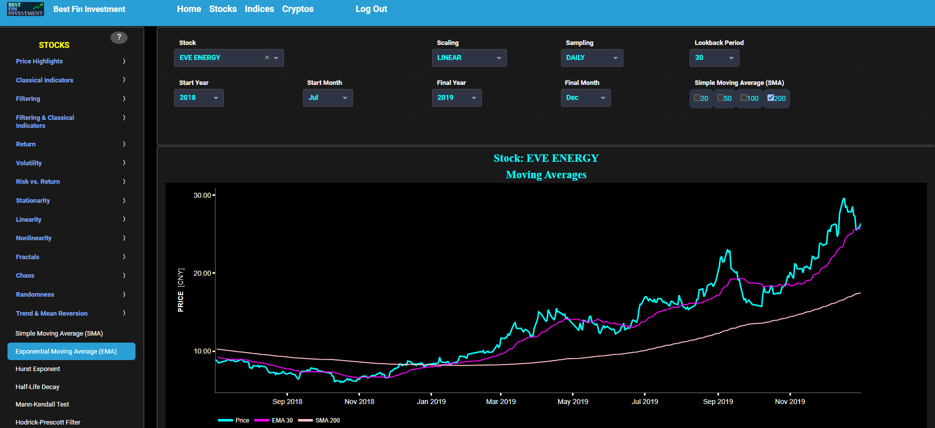
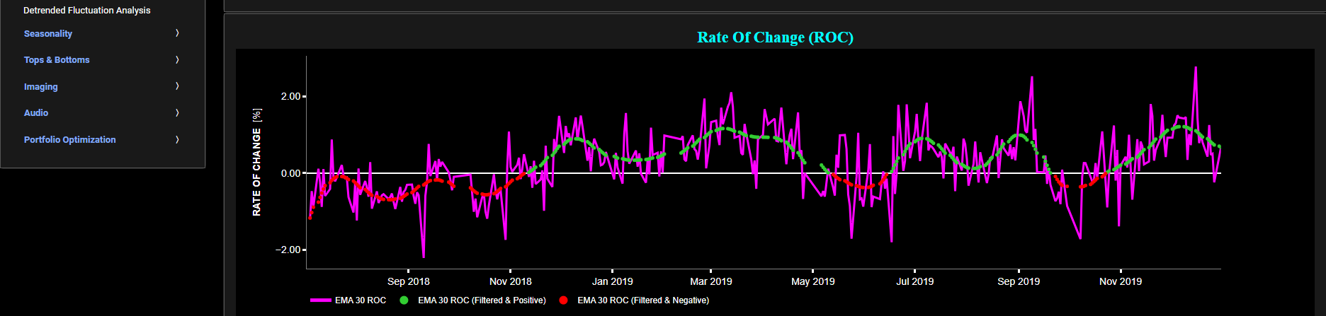
Trend & Mean Reversion
Relative Strength Index
This page visualizes historical asset prices in cyan color using either daily, weekly, or monthly close prices. In the menu bar (located just above the graphs), you can also select specific time periods to visualize and also toggle between a linear or logarithmic price scaling on the left y-axis. In addition the graph allows you to superimpose several Simple Moving Average (SMA) lines. Next to the asset price line in cyan color, the graph also visualizes the asset price Relative Strength Index (RSI) in magenta, and the RSI for a synthetically generated random walk in yellow. In a random walk, each step is independent of the previous steps, and there is no systematic trend or pattern in the data. The random walk data points are given here for reference and comparison purposes (i.e. benchmarking).
The RSI is computed using a lookback time period that is selected in the menu bar (located just above the graphs). Typically a lookback value of 14 is selected. Next the white line represents a filtered version of the magenta line through the application of a low-pass Butterworth digital filter. The RSI is a so-called momentum metric that measures the change of asset price movements, helping to identify overbought or oversold conditions. Developed by J. Welles Wilder, RSI is widely used in technical analysis to assess the strength and direction of price trends.
The RSI interpretation is given as follows: traditionally, an RSI above 70 is considered overbought, suggesting that the asset may be due for a price correction or a reversal. Conversely, an RSI below 30 is considered oversold, indicating that the asset might be undervalued and due for a potential price increase or a reversal. RSI can further provide additional information about price patterns, trends and potential reversals. The so-called divergence patterns occur when RSI and price movements do not confirm each other, indicating a potential price trend reversal. For example, if the price makes a new high but the RSI doesn't, it may suggest weakness in the uptrend (i.e. bearish divergence). Similarly when the price makes new lows while the RSI doesn't may suggest a potential upward reversal (i.e. bullish divergence).
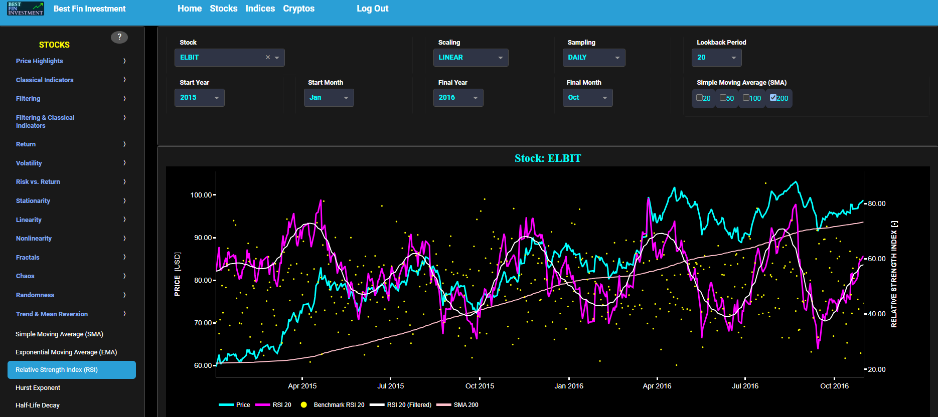
Trend & Mean Reversion
Hurst Exponent
This page visualizes historical asset prices in cyan color using either daily, weekly, or monthly close prices. In the menu bar (located just above the graphs), you can also select specific time periods to visualize and also toggle between a linear or logarithmic price scaling on the left y-axis. In addition the graph allows you to superimpose several Simple Moving Average (SMA) lines. Next to the asset price line in cyan color, the graph also visualizes the Hurst Exponent (HE) statistical measure computed using the R/S statistic.
The HE, named after the British hydrologist Harold Edwin Hurst (1880 – 1978), is used in various fields, including hydrology, to assess long-range dependence or persistence in time series data. In the context of hydrology, the HE is often used to analyze and understand the behavior of hydrological processes, particularly the flow of water in rivers, streams, and other water bodies. Essentially the HE helps to understand whether the flow at a particular time is influenced by past flow measurements over extended periods, i.e. the long-range dependence or memory of river flow. Similarly in financial time series analysis, the HE may be used to analyze the intrinsic behavior of the asset's price movements. When applied to asset prices, the HE helps analyze whether the asset's prices exhibit a trending (persistent) or ean-reverting (anti-persistent) behavior. The graph shows the asset price HE in magenta, and the HE for a synthetically generated random walk in yellow. In a random walk, each step is independent of the previous steps, and there is no systematic trend or pattern in the data. The random walk data points are given here for reference and comparison purposes (i.e. benchmarking). The HE is computed using a lookback time period that is selected in the menu bar (located just above the graphs). Next the white line represents a filtered version of the magenta line through the application of a low-pass Butterworth digital filter.
Finally the HE interpretation is given as follows: A HE < 0.5 indicates a mean-reverting or anti-persistent behavior. In the context of asset prices, it suggests that the asset tends to revert to its mean price over time. This could imply opportunities for contrarian strategies. A HE > 0.5 suggests a trending or persistent behavior, indicating that the asset exhibits long-term trends and momentum. A HE value around 0.5 suggests a random walk.
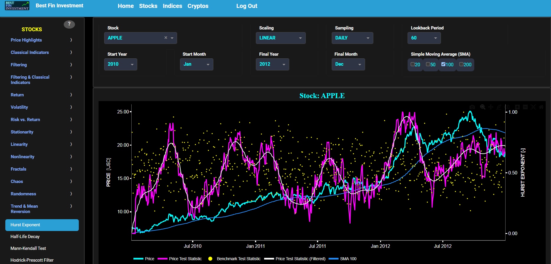
Trend & Mean Reversion
Half-Life Decay
This page visualizes historical asset prices in cyan color using either daily, weekly, or monthly close prices. In the menu bar (located just above the graphs), you can also select specific time periods to visualize and also toggle between a linear or logarithmic price scaling on the left y-axis. In addition the graph allows you to superimpose several Simple Moving Average (SMA) lines. Next to the asset price line in cyan color, the graph also visualizes the Half-Life Decay (HLD) statistical metric which quantifies the mean reversion in a financial time series based on a linear regression model.
The HLD can be used to assess whether the asset price follows a mean-reverting or trend-following behavior. The graph shows the asset price HLD in magenta, and the HLD for a synthetically generated random walk in yellow. In a random walk, each step is independent of the previous steps, and there is no systematic trend or pattern in the data. The random walk data points are given here for reference and comparison purposes (i.e. benchmarking). The HLD is computed using a lookback time period that is selected in the menu bar (located just above the graphs). Next the white line represents a filtered version of the magenta line through the application of a low-pass Butterworth digital filter. Finally the HLD interpretation is given as follows: if HLD is a small value, it implies that the time series reverts to its mean relatively quickly, indicating a strong mean-reverting behavior. This might suggest that the asset exhibits short-term trends. On the other hand, a large HLD value suggests a slower mean reversion, indicating that the time series tends to exhibit longer-term trends.
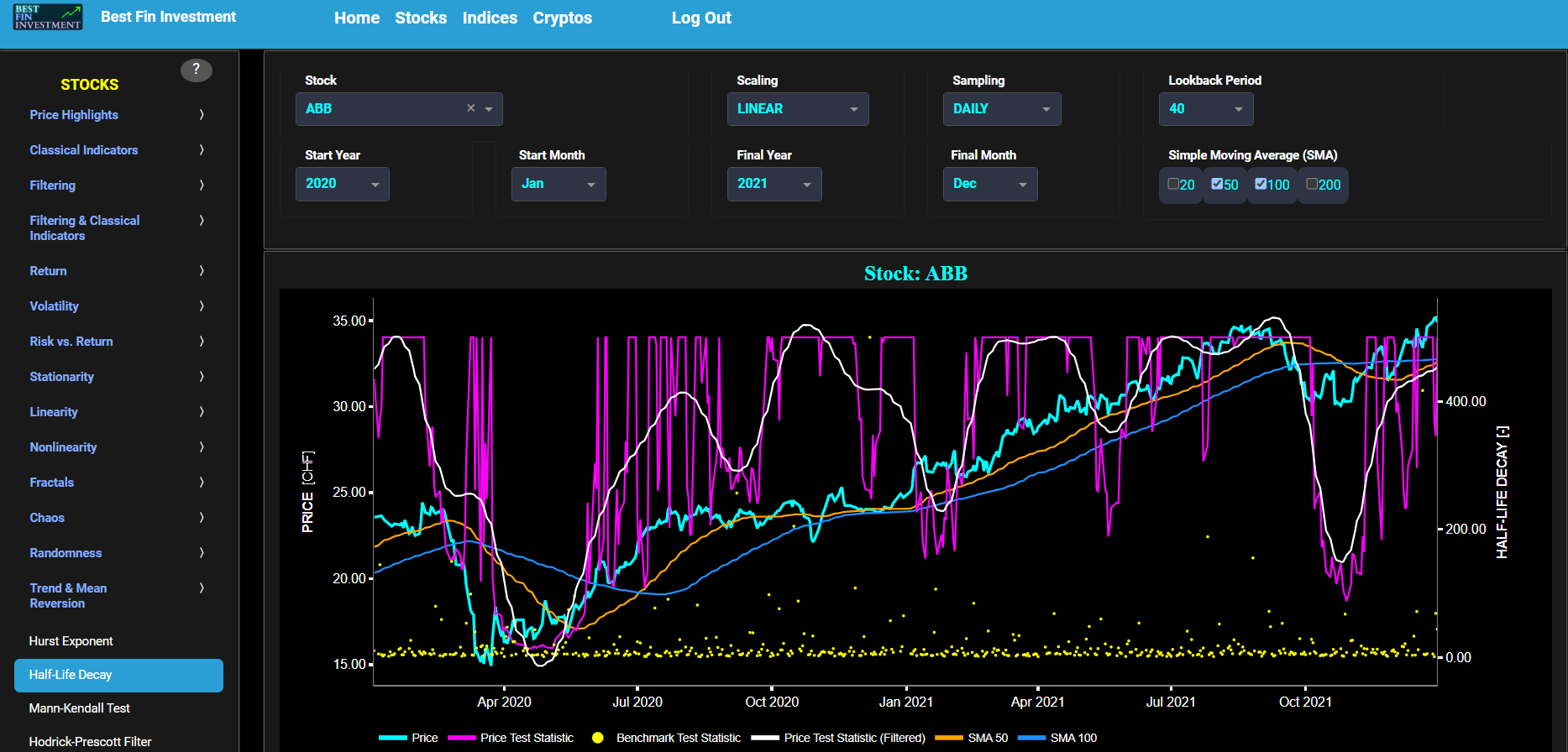
Trend & Mean Reversion
Mann-Kendall Test
This page provides 2 graphs. The upper graph visualizes historical asset prices in cyan color using either daily, weekly, or monthly close prices. In the menu bar (located just above the graphs), you can also select specific time periods to visualize and also toggle between a linear or logarithmic price scaling on the left y-axis. In addition the upper graph allows you to superimpose several Simple Moving Average (SMA) lines. Next to the asset price line in cyan color, the graph also visualizes the statistic of the Mann-Kendall (MK) trend test.
The MK is a non-parametric statistical test used to detect trends in time series data. In our case the graph shows the so-called MK Tau value which is a measure of the strength and direction of the trend. The graph shows the asset price MK Tau value in magenta and the MK Tau value for a synthetically generated random walk in yellow. In a random walk, each step is independent of the previous steps, and there is no systematic trend or pattern in the data. The random walk data points are given here for reference and comparison purposes (i.e. benchmarking). The MK Tau is computed using a lookback time period that is selected in the menu bar (located just above the graphs). Next the white line represents a filtered version of the magenta line through the application of a low-pass Butterworth digital filter. Finally the MK Tau interpretation is given as follows: if the Tau value is positive, it indicates a positive trend, while a negative tau value represents a negative trend. The absolute value of the Tau value is a measure of the strength of the trend.
Next the lower graph visualizes the statistical significance (p-value) of the MK test for the asset return in magenta, and for the benchmark signal in yellow. The p-value associated with the MK statistic indicates the probability of obtaining a test statistic as extreme as the one observed if the null hypothesis were true. A small p-value (typically less than a significance level, e.g., 0.05) suggests that the observed trend is statistically significant.
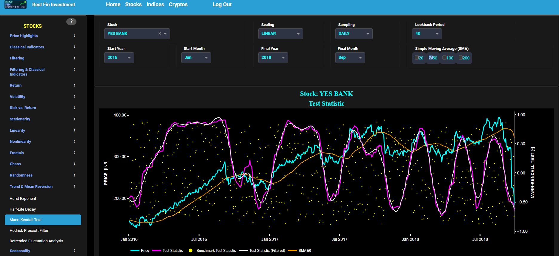
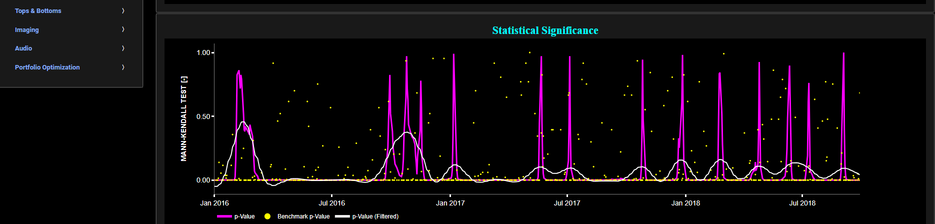
Trend & Mean Reversion
Hodrick-Prescott Filter
This page provides 2 graphs. The upper graph visualizes historical asset prices in cyan color using either daily, weekly, or monthly close prices. In the menu bar (located just above the graphs), you can also select specific time periods to visualize and also toggle between a linear or logarithmic price scaling on the left y-axis. In addition the upper graph allows you to superimpose several Simple Moving Average (SMA) lines. Next to the asset price line in cyan color, the upper graph also visualizes a magenta line which is the trend line from the Hodrick-Prescott (HP) filter.
The HP filter is known as a common time series decomposition method and is computed using a lookback time period that is selected in the menu bar (located just above the graphs). By separating the time series into two components (trend + cycle), the HP filter allows to analyze and interpret an asset's price behavior in terms of both its long-term trends and its shorter-term cyclical movements. The HP trend line filters out short-term fluctuations and noise, revealing the smoother, longer-term price direction. The lower graph visualizes the HP filter cycle component which represents the cyclical, short-term, or oscillatory behavior in the asset price time series. It captures the deviations from the long-term trend, which can be attributed to shorter-term market dynamics, cycles, or other irregular fluctuations.
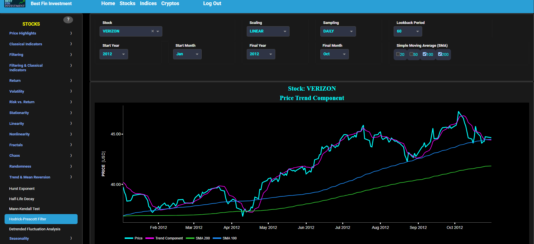
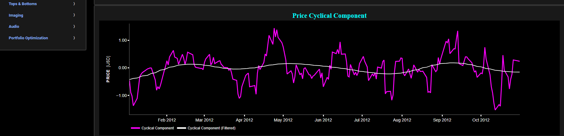
Trend & Mean Reversion
Detrended Fluctuation Analysis
This page provides 2 graphs. The upper graph visualizes historical asset prices in cyan color using either daily, weekly, or monthly close prices. In the menu bar (located just above the graphs), you can also select specific time periods to visualize and also toggle between a linear or logarithmic price scaling on the left y-axis. In addition the upper graph allows you to superimpose several Simple Moving Average (SMA) lines. Next to the cyan line, the upper graph also visualizes the Detrended Fluctuation Analysis (DFA) scaling exponent for the asset price in magenta and for a synthetically generated random walk in yellow color. In a random walk, each step is independent of the previous steps, and there is no systematic trend or pattern in the data. The yellow random walk data points are given here for reference and comparison purposes (i.e. benchmarking).
The DFA is a method used to analyze long-range correlations and scaling behavior in time series data. It was originally introduced in the field of statistical physics to study the statistical properties of complex physical systems, particularly those exhibiting self-similarity and fractal-like behavior. It was later applied to various disciplines, including finance, biology, and geophysics. Now in the context of financial time series analysis, the DFA can help identify whether the asset price data shows long-range dependencies and whether it follows a random walk, has trending behavior, or exhibits mean-reversion. Here the DFA is computed using a lookback time period that is selected in the menu bar (located just above the graphs). Next the white line represents a filtered version of the magenta line through the application of a low-pass Butterworth digital filter. The DFA is a generalization of the Hurst exponent, and in terms of DFA interpretation we have the following: a DFA value < 0.5 suggests anti-correlation (i.e. mean-reversion), a DFA value around 0.5 indicates no correlation (i.e. white noise), a DFA value > 0.5 suggests correlation (i.e. trend), a DFA value around 1.0 indicates a so-called 1/f-noise (i.e. pink noise), a DFA value > 1.0 suggests non-stationarity and unboundedness, a DFA value around 1.5 indicates Brownian noise (i.e. random walk), and a DFA value > 1.5 may suggest an unusual or complex behavior, indicating that the data does not conform to the standard DFA model and could have unique characteristics not captured by our DFA model.
Regarding the lower graph, this latter visualizes the asset price in cyan color, and the DFA value for the asset incremental return in magenta together with the DFA value for a benchmark signal in yellow. Incremental return is defined as the percentage change in the asset's price between consecutive time periods, whereas the benchmark signal is based upon synthetically generated, normally distributed, independent and identically distributed (i.i.d.) returns. For this benchmark signal, each step is independent of the previous steps, and there is no systematic trend or pattern in the data.
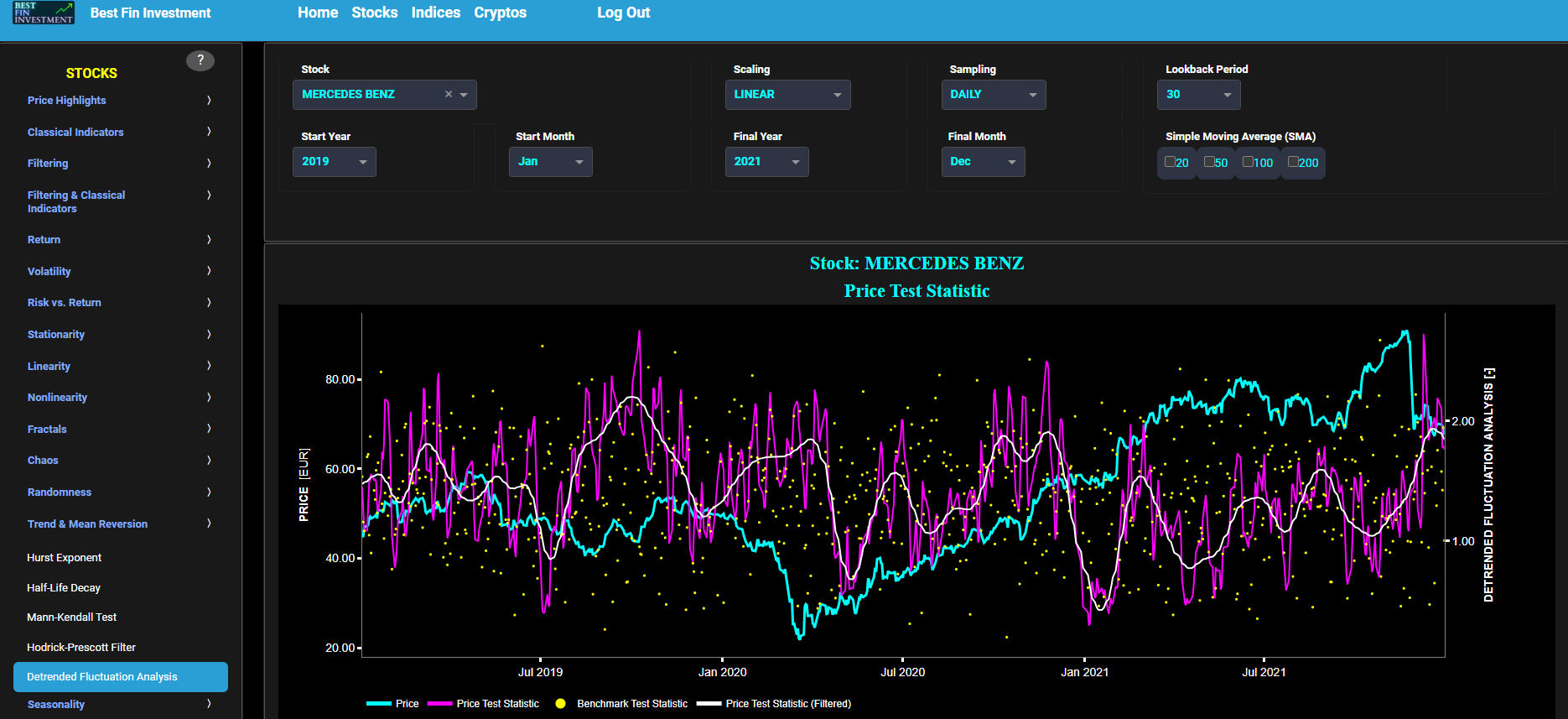
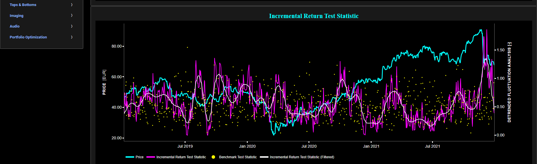
Seasonality
Day Of Week
This page provides 2 graphs. The upper graph visualizes historical asset prices in cyan color using either daily, weekly, or monthly close prices. In the menu bar (located just above the graphs), you can also select specific time periods to visualize and also toggle between a linear or logarithmic price scaling on the left y-axis. Next to the cyan line, the upper graph also visualizes incremental return in magenta color. Here incremental return is defined as the % change between 2 consecutive close prices. The lower graph visualizes the cumulative return for each Day Of Week separately. This may help reveal insights into investor’s behavior and identify potential seasonality patterns.
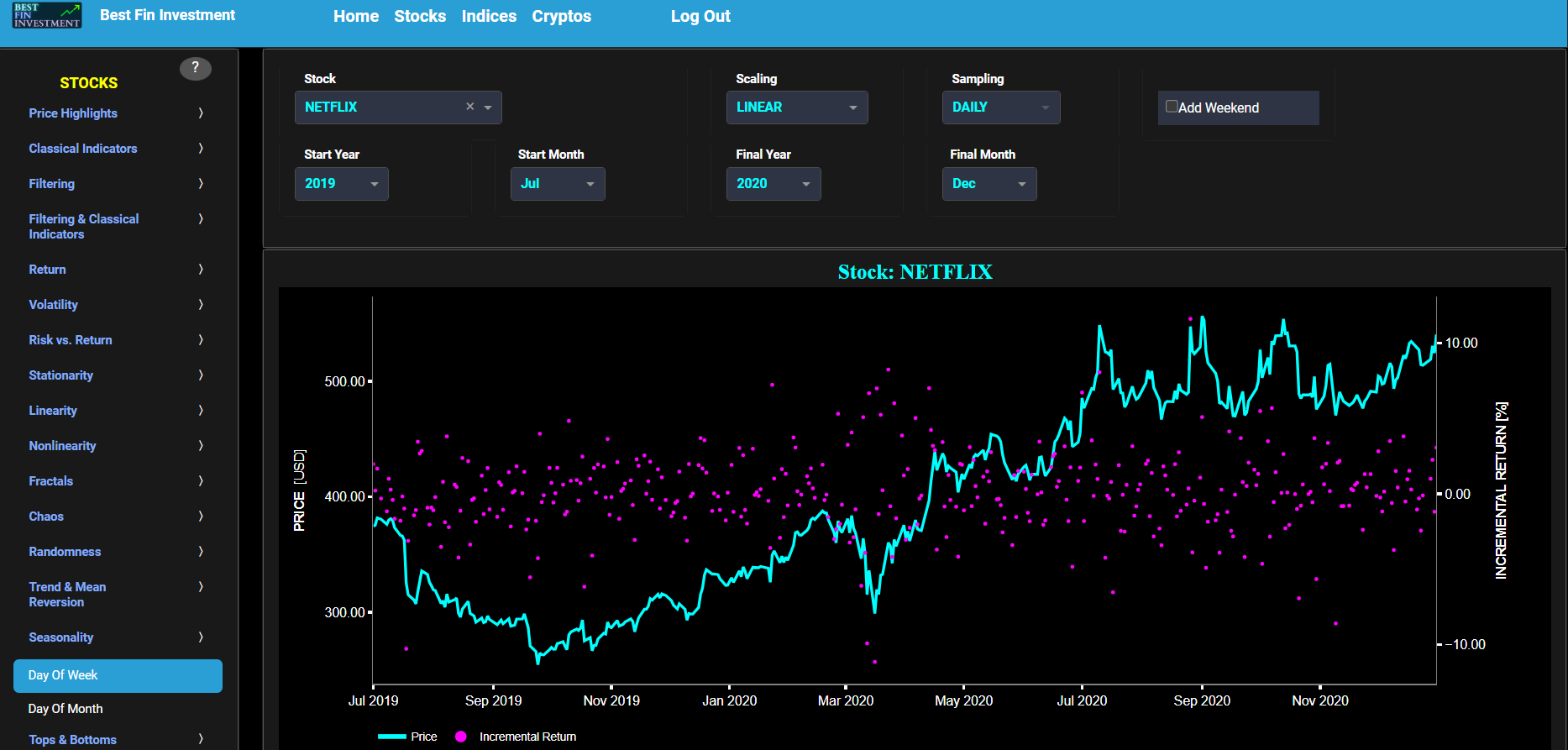
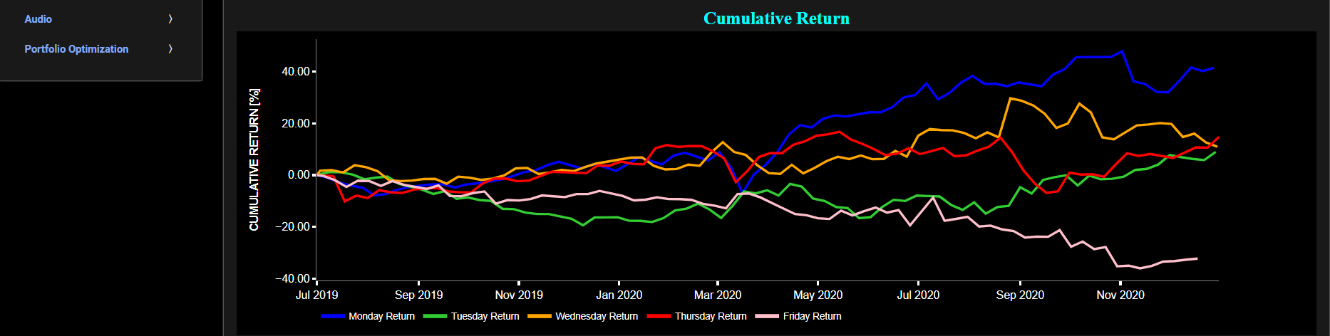
Seasonality
Day Of Month
This page provides 2 graphs. The upper graph visualizes historical asset prices in cyan color using either daily, weekly, or monthly close prices. In the menu bar (located just above the graphs), you can also select specific time periods to visualize and also toggle between a linear or logarithmic price scaling on the left y-axis. Next to the cyan line, the upper graph also visualizes incremental return in magenta color. Here incremental return is defined as the % change between 2 consecutive close prices. Further you can also select up to 4 specific Day Of Month time periods for comparisons of cumulative return. The lower graph visualizes the cumulative return for each of the 4 Day Of Month periods separately. This may help reveal insights into investor’s behavior and identify potential seasonality patterns.
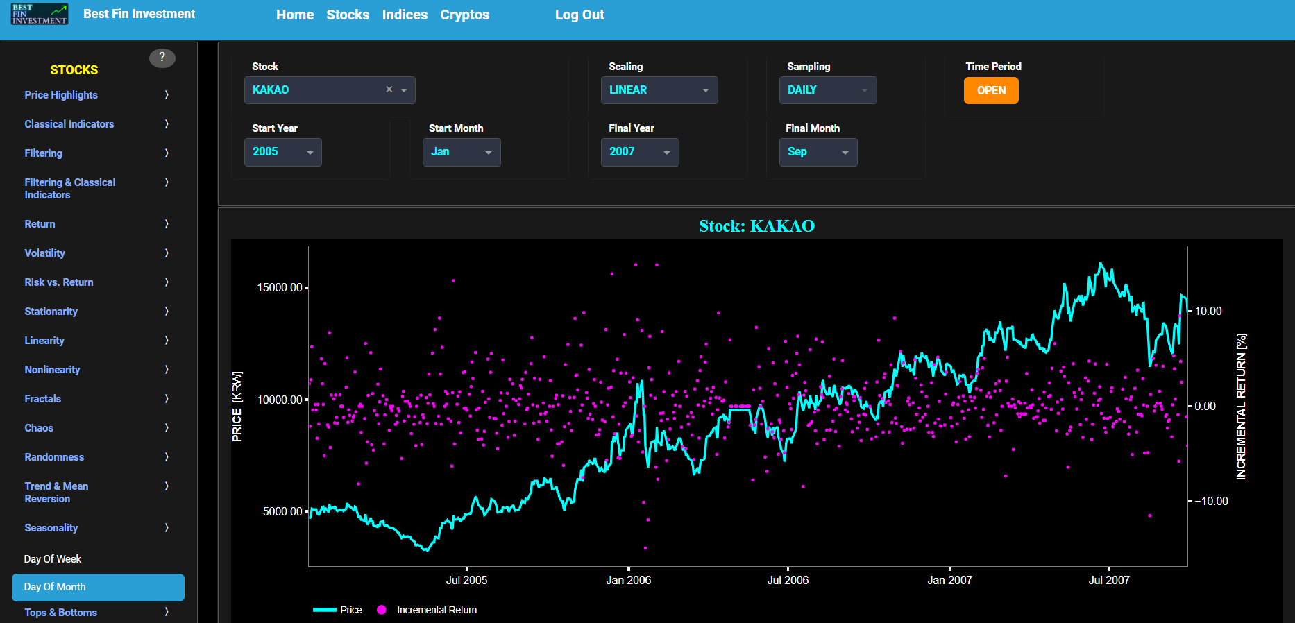
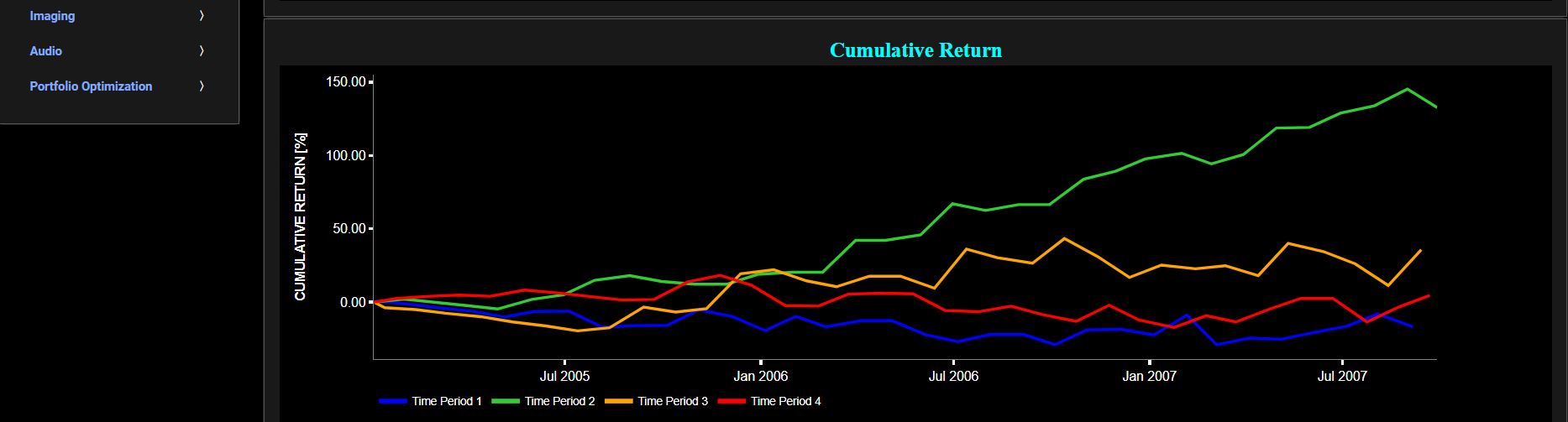
Tops & Bottoms
Log Periodic Power Law Singularity (LPPLS) Model
This page visualizes historical asset prices in cyan color using daily close prices. In the menu bar (located just above the graphs), you can also select specific time periods to visualize and also toggle between a linear or logarithmic price scaling on the left y-axis. The graph also shows potential market tops (in red color dots) and bottoms (in green color dots) using the Log Periodic Power Law Singularity (LPPLS) Model. In the menu bar (located just above the graph) you can adjust the model sensitivity by selecting specific values for the detection thresholds of market tops and bottoms respectively (regarding the model rolling window size, it has been set to a default value of 20).
The LPPLS model is a mathematical framework used to describe the behavior of financial market bubbles and predict potential market critical points, and was developed by Prof. Didier Sornette and his research group. Sornette’s group has conducted research since the mid 1990s in various fields including: seismology, earthquake and rupture prediction, statistical physics, complex systems theory, and financial market bubbles and crashes. Inspired by earthquake prediction models, the LPPLS model considers the faster-than-exponential (i.e. power law) increase in asset prices decorated by accelerating oscillations as the main diagnostic of financial market bubbles. Essentially it models the effect of positive feedback loops of higher return anticipations competing with negative feedback spirals of crash expectations. Sornette's work emphasizes the interdisciplinary nature of financial market analysis, combining tools from physics, mathematics, and economics to gain a better understanding of market dynamics.
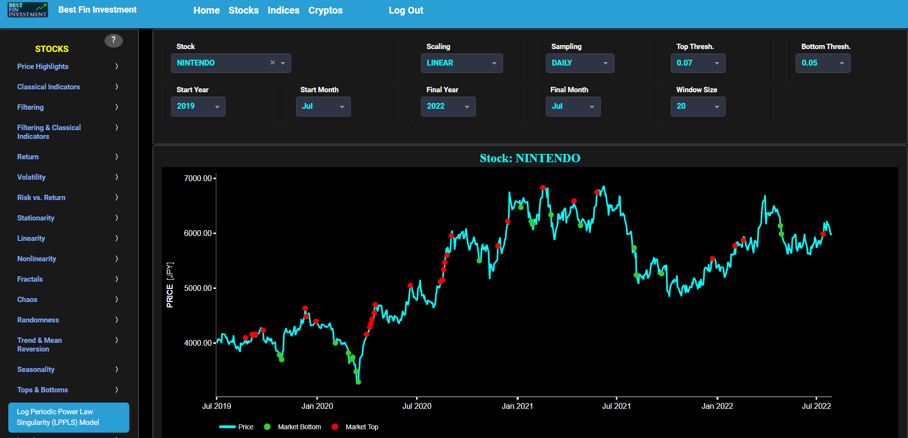
Econophysics
Agent-Based Model (ABM)
Econophysics emerged in the mid-1990s as an interdisciplinary field applying principles and methodologies from physics to analyze economic and financial systems. An illustrative instance is the phenomenon of volatility clustering observed in financial markets, reminiscent of the intermittent dynamics seen in complex physical systems like velocity fluctuations in turbulent flows and avalanche dynamics. Pioneering figures in econophysics include Jean-Philippe Bouchaud, J. Doyne Farmer, Rosario Mantegna, Didier Sornette, and Eugene Stanley.
Traditional economic theories tended to favor simplified, closed-form models for theoretical convenience, often neglecting empirical validation. Standard economic models typically assumed rational, homogeneous agents operating within equilibrium conditions. However, empirical evidence demonstrated that the complex dynamics of financial markets were heavily influenced by interactions among heterogeneous agents, leading to non-equilibrium market conditions.
Agent-Based Models (ABM) are numerical simulations featuring autonomous decision-making entities known as agents. ABM are particularly intriguing as they illustrate how simple interactions at the micro level can give rise to complex patterns at the macro level, such as crowd behavior. In other words, the whole (i.e. market dynamics) is fundamentally different from any of its elementary sub-parts. In nonlinear complex systems like financial markets, small disturbances at the micro level can lead to significant fluctuations at the macro level, whereas large disturbances at the micro level may not necessarily produce equally large fluctuations at the macro level.
ABM have been instrumental in explaining several statistical regularities observed in financial time series, known as stylized facts, including fat tails, excess volatility, volatility clustering, trend following, mean reversion, temporary bubbles, sudden crashes, and markets in a perpetual transient state. Market volatility, in particular, is understood to be primarily endogenous, influenced by trading activity and associated feedback loops, rather than solely driven by rational responses to exogenous news. This insight suggests that self-generated high-frequency price movements play a substantial role in market dynamics. In contrast, lower-frequency price movements may be more influenced by external factors such as exogenous macro news or exogenous news related to business fundamental value.
Now this page provides 2 graphs. The upper graph visualizes historical asset prices, on the left y-axis, in cyan color using either daily, weekly, or monthly close prices. In the menu bar (located just above the graphs), you can also select specific time periods to visualize and also toggle between a linear or logarithmic price scaling on the y-axes. In addition the upper graph also visualizes the output of an ABM, on the right y-axis, in magenta color.
We use a simplified ABM to simulate the dynamics of a financial market. The model consists of a predefined number of N agents (which can be selected in the top menu bar), each of which makes binary decisions to either buy or sell the selected asset at each time step. To be more specific, we define a binary decision variable D_i for each agent i as follows: D_i = 0 indicates agent i is selling the asset, and D_i = 1 indicates that agent i is buying the asset. Next we define an agent’s behavior B_i as: B_i = alpha_i + beta_i * M, where alpha_i represents the agent’s personal opinion of long-term returns and beta_i the Incentive due to social or peer pressure. However In our model, we use a very simple ABM in which all agents have identical alpha and beta coefficients, namely alpha = alpha_i for all agents i and beta = beta_i for all agents i. These alpha and beta coefficients can be adjusted in the top menu bar. Note that despite the uniformity in alpha and beta coefficients across all agents in our model, each agent still exhibits unique behavior due to the probabilistic framework used to translate this behavior into buy or sell decisions.
Now the variable M represents the average of all agent decisions, i.e. the Market. Next we have a probabilistic decision theory framework where the probability of an agent i switching from selling to buying P_i(0 -> 1) is calculated using: P_i(0 -> 1) = exp(B_i) / (1 + exp(B_i)). Finally, we use a binomial distribution to convert probabilities P_i into decision variable D_i. Now the model is basically a simulation that iterates over each time step, updating the decisions D_i of each agent i, based on their calculated behavior and probabilistic decision-making. The average of all agents' decisions over time is plotted as the magenta line, reflecting the collective behavior and dynamics of a financial market under the specified parameters that you have selected in the top menu bar. In particular such a plot allows one to visualize the endogenous dynamics and volatility clustering of a financial market.
Regarding the lower graph, this latter visualizes the incremental return of the selected asset in cyan color, and the incremental return of the ABM in magenta color.
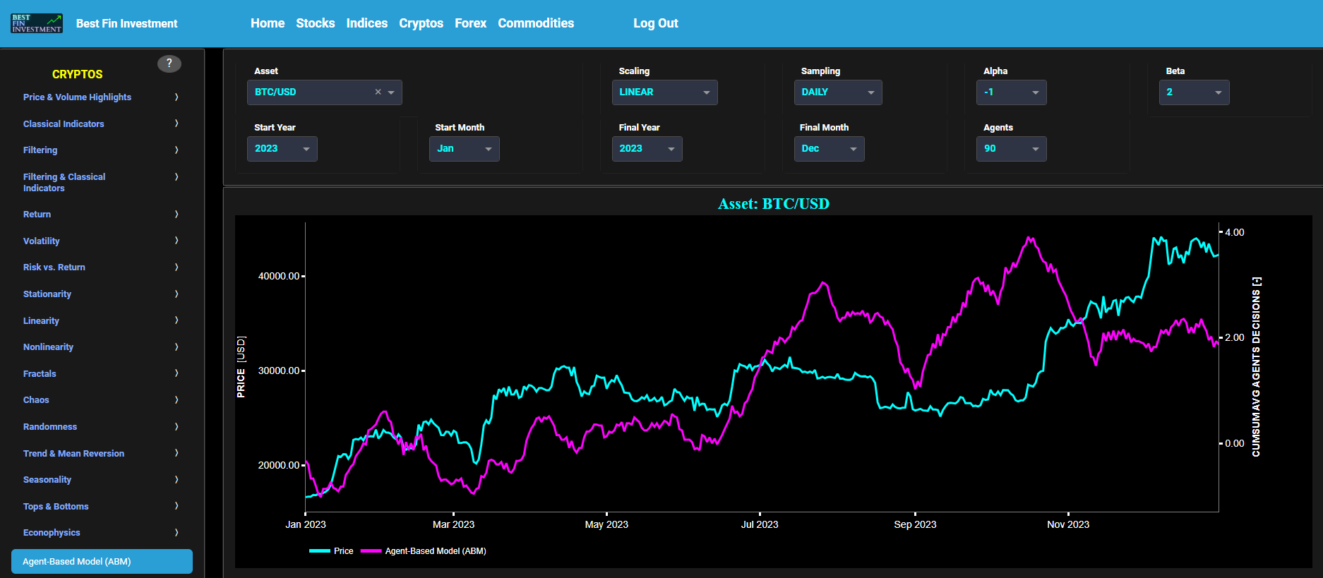
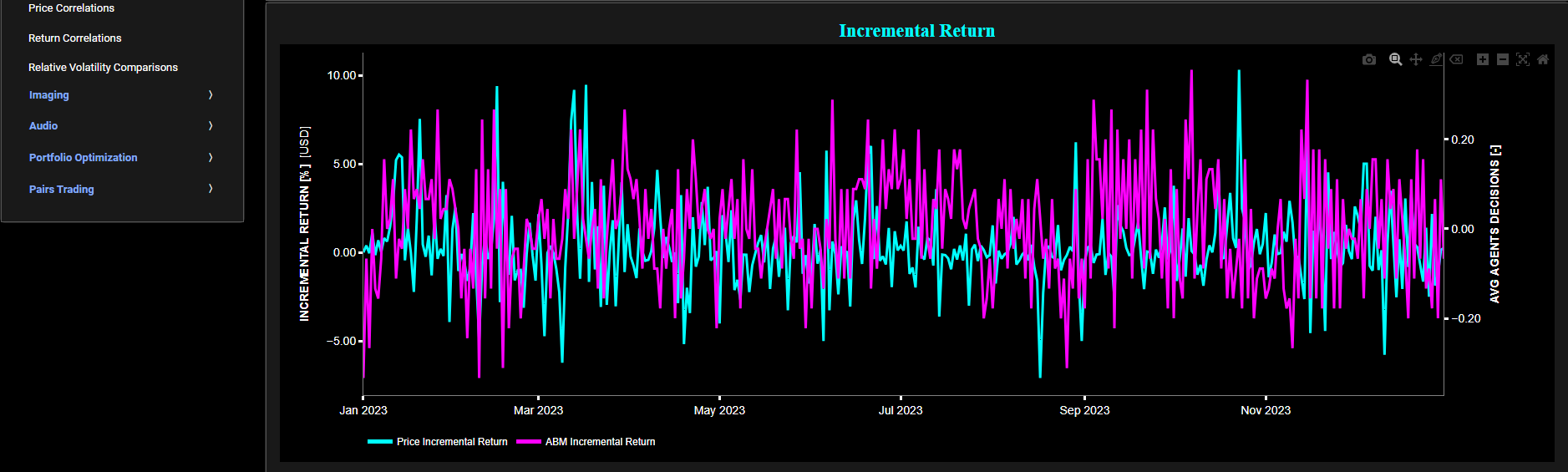
Econophysics
ABM: Price Correlations
The purpose of this page is to find Agent-Based Models (ABM) that best approximate the observed asset price trajectory. ABM are numerical simulations featuring autonomous decision-making entities known as agents. ABM are particularly intriguing as they illustrate how simple interactions at the micro level can give rise to complex patterns at the macro level. We use a simplified ABM to simulate the dynamics of a financial market. The model consists of a predefined number of N agents (which can be selected in the top menu bar), each of which makes binary decisions to either buy or sell the selected asset at each time step. Now an agent’s behavior B_i is defined as follows: B_i = alpha_i + beta_i * M, where alpha_i represents the agent’s personal opinion of long-term returns and beta_i the Incentive due to social or peer pressure. However In our model, we use a very simple ABM in which all agents have identical alpha and beta coefficients, namely alpha = alpha_i for all agents i and beta = beta_i for all agents i.
Note that despite the uniformity in alpha and beta coefficients across all agents in our model, each agent still exhibits unique behavior due to the probabilistic framework used to translate this behavior into buy or sell decisions. For more information please refer also to the page “Agent-Based Model (ABM)”.
The goal is now to find the optimal parameters (alpha and beta) of an ABM model such that the correlation between the ABM’s price dynamics and the observed asset price data is maximized. This optimization process is repeated multiple times. The top menu bar allows you to also select one of three correlation metrics: Pearson, Spearman, and Kendall-Tau.
This page provides 2 graphs. The upper graph visualizes historical asset prices in cyan color using either daily, weekly, or monthly close prices. In the menu bar (located just above the graphs), you can also select specific time periods to visualize and also toggle between a linear or logarithmic price scaling on the left y-axis. The lower graph shows the optimal alpha and beta ABM coefficient values, presented in a so-called distribution violin plot.
Now patterns in the distributions of alpha and beta coefficients can reveal information about price momentum and trend-following behavior in the market. Clusters of high alpha and beta values may indicate periods of strong upward momentum, while low alpha and beta values may suggest a lack of conviction or trend reversal.
For example the analysis of the distribution of optimal alpha coefficients may provide insights into the prevailing market sentiment regarding the selected asset. Higher values of alpha may indicate a bullish sentiment among investors, suggesting optimism about future price movements. Conversely, lower alpha values may signal a bearish sentiment or skepticism about the asset's prospects.
Furthermore, by examining the distribution of optimal beta coefficients, we may be able to assess the degree of herding behavior or market influence among investors. A higher beta implies that investors are more susceptible to external factors and market trends, potentially leading to increased volatility and herd-like behavior in trading decisions.
Finally the variability in the distributions of alpha and beta coefficients may provide insights into market volatility expectations. Wide distributions or high levels of dispersion may potentially suggest heightened uncertainty and volatility in the market, while narrow distributions may indicate relatively stable market conditions.
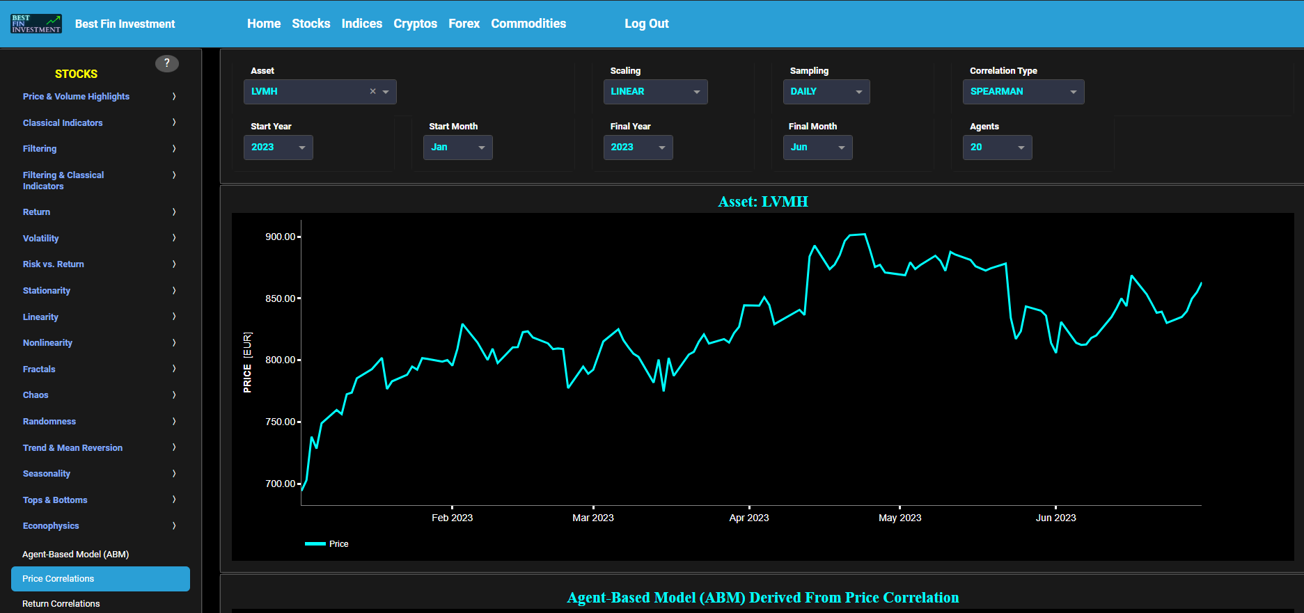
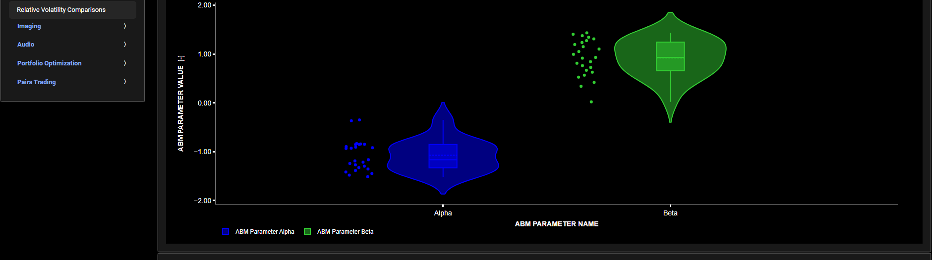
Econophysics
ABM: Return Correlations
The purpose of this page is to find Agent-Based Models (ABM) that best approximate the observed asset incremental return trajectory. ABM are numerical simulations featuring autonomous decision-making entities known as agents. ABM are particularly intriguing as they illustrate how simple interactions at the micro level can give rise to complex patterns at the macro level. We use a simplified ABM to simulate the dynamics of a financial market. The model consists of a predefined number of N agents (which can be selected in the top menu bar), each of which makes binary decisions to either buy or sell the selected asset at each time step. Now an agent’s behavior B_i is defined as follows: B_i = alpha_i + beta_i * M, where alpha_i represents the agent’s personal opinion of long-term returns and beta_i the Incentive due to social or peer pressure. However In our model, we use a very simple ABM in which all agents have identical alpha and beta coefficients, namely alpha = alpha_i for all agents i and beta = beta_i for all agents i.
Note that despite the uniformity in alpha and beta coefficients across all agents in our model, each agent still exhibits unique behavior due to the probabilistic framework used to translate this behavior into buy or sell decisions. For more information please refer also to the page “Agent-Based Model (ABM)”.
The goal is now to find the optimal parameters (alpha and beta) of an ABM model such that the correlation between the ABM’s incremental return dynamics and the observed asset incremental return data is maximized. This optimization process is repeated multiple times. The top menu bar allows you to also select one of three correlation metrics: Pearson, Spearman, and Kendall-Tau.
This page provides 2 graphs. The upper graph visualizes historical asset prices in cyan color using either daily, weekly, or monthly close prices. In the menu bar (located just above the graphs), you can also select specific time periods to visualize and also toggle between a linear or logarithmic price scaling on the left y-axis. The lower graph shows the optimal alpha and beta ABM coefficient values, presented in a so-called distribution violin plot.
Now patterns in the distributions of alpha and beta coefficients can reveal information about price momentum and trend-following behavior in the market. Clusters of high alpha and beta values may indicate periods of strong upward momentum, while low alpha and beta values may suggest a lack of conviction or trend reversal.
For example the analysis of the distribution of optimal alpha coefficients may provide insights into the prevailing market sentiment regarding the selected asset. Higher values of alpha may indicate a bullish sentiment among investors, suggesting optimism about future price movements. Conversely, lower alpha values may signal a bearish sentiment or skepticism about the asset's prospects.
Furthermore, by examining the distribution of optimal beta coefficients, we may be able to assess the degree of herding behavior or market influence among investors. A higher beta implies that investors are more susceptible to external factors and market trends, potentially leading to increased volatility and herd-like behavior in trading decisions.
Finally the variability in the distributions of alpha and beta coefficients may provide insights into market volatility expectations. Wide distributions or high levels of dispersion may potentially suggest heightened uncertainty and volatility in the market, while narrow distributions may indicate relatively stable market conditions.
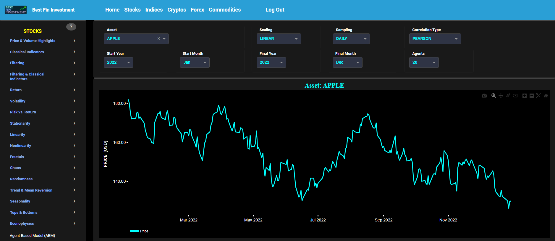
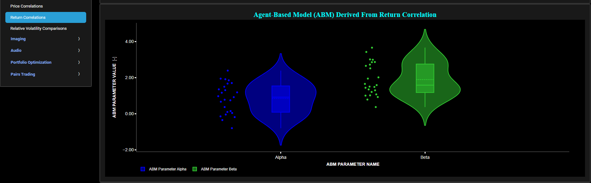
Econophysics
ABM: Relative Volatility Comparisons
The purpose of this page is to find Agent-Based Models (ABM) that best approximate the observed asset relative volatility. In our case we define relative volatility as the Coefficient of Variation (CV), i.e. the ratio of the standard deviation to the mean of a price data set. ABM are numerical simulations featuring autonomous decision-making entities known as agents. ABM are particularly intriguing as they illustrate how simple interactions at the micro level can give rise to complex patterns at the macro level. We use a simplified ABM to simulate the dynamics of a financial market. The model consists of a predefined number of N agents (which can be selected in the top menu bar), each of which makes binary decisions to either buy or sell the selected asset at each time step. Now an agent’s behavior B_i is defined as follows: B_i = alpha_i + beta_i * M, where alpha_i represents the agent’s personal opinion of long-term returns and beta_i the Incentive due to social or peer pressure. However In our model, we use a very simple ABM in which all agents have identical alpha and beta coefficients, namely alpha = alpha_i for all agents i and beta = beta_i for all agents i.
Note that despite the uniformity in alpha and beta coefficients across all agents in our model, each agent still exhibits unique behavior due to the probabilistic framework used to translate this behavior into buy or sell decisions. For more information please refer also to the page “Agent-Based Model (ABM)”.
The goal is now to find the optimal parameters (alpha and beta) of an ABM model such that the absolute difference between the ABM’s relative volatility and the observed relative volatility is minimized. This optimization process is repeated multiple times.
This page provides 2 graphs. The upper graph visualizes historical asset prices in cyan color using either daily, weekly, or monthly close prices. In the menu bar (located just above the graphs), you can also select specific time periods to visualize and also toggle between a linear or logarithmic price scaling on the left y-axis. The lower graph shows the optimal alpha and beta ABM coefficient values, presented in a so-called distribution violin plot.
The optimal alpha and beta coefficients obtained through this minimization process may provide insights into the degree of optimism/pessimism among all agents (alpha) and the influence of social interactions on decision-making (beta), adjusted to better match the observed asset (i.e. market) volatility. These coefficients reflect the collective behavior of agents within the ABM framework and hence their impact on asset price movements.
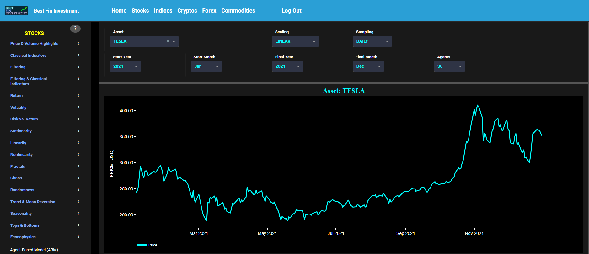
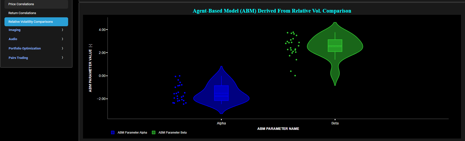
Imaging
Wavelet Spectrogram
This page provides 2 graphs. The upper graph visualizes historical asset prices in cyan color using either daily, weekly, or monthly close prices. In the menu bar (located just above the graphs), you can also select specific time periods to visualize and also toggle between a linear or logarithmic price scaling on the left y-axis. Next to the cyan line, the upper graph also visualizes incremental return in magenta color. Here incremental return is defined as the % change between 2 consecutive close prices.
The lower graph visualizes a Continuous Wavelet Transform (CWT) for the selected asset price. CWT are powerful tools for time-frequency analysis and have been widely used in various fields, including: signal processing, geophysics, medical imaging, image processing, and finance. In finance CWT can help identify patterns, cycles and fluctuations that might not be evident in a simple time series plot. These can further be used to detect sudden changes in market behavior.
In the top menu bar you can also toggle between 4 Wavelet forms, namely: Morlet, Complex Morlet, Gaussian, and Mexican Hat wavelets. These have the following characteristics. The Morlet Wavelet is known to be a good general-purpose wavelet, offering good frequency localization, and is suitable for analyzing signals with both high and low frequencies. The Complex Morlet Wavelet also offers good time and frequency localization, is useful for analyzing non-stationary signals and detecting oscillatory patterns, and can capture both high and low-frequency components effectively. The Gaussian Wavelet provides smooth and continuous wavelet transforms, is suitable for analyzing signals with Gaussian-like characteristics, and is useful for noise reduction and feature extraction tasks. Finally the Mexican Hat Wavelet provides good time and frequency localization, is suitable for detecting transient features and sharp changes in a signal, and is often used in detecting edges and discontinuities.
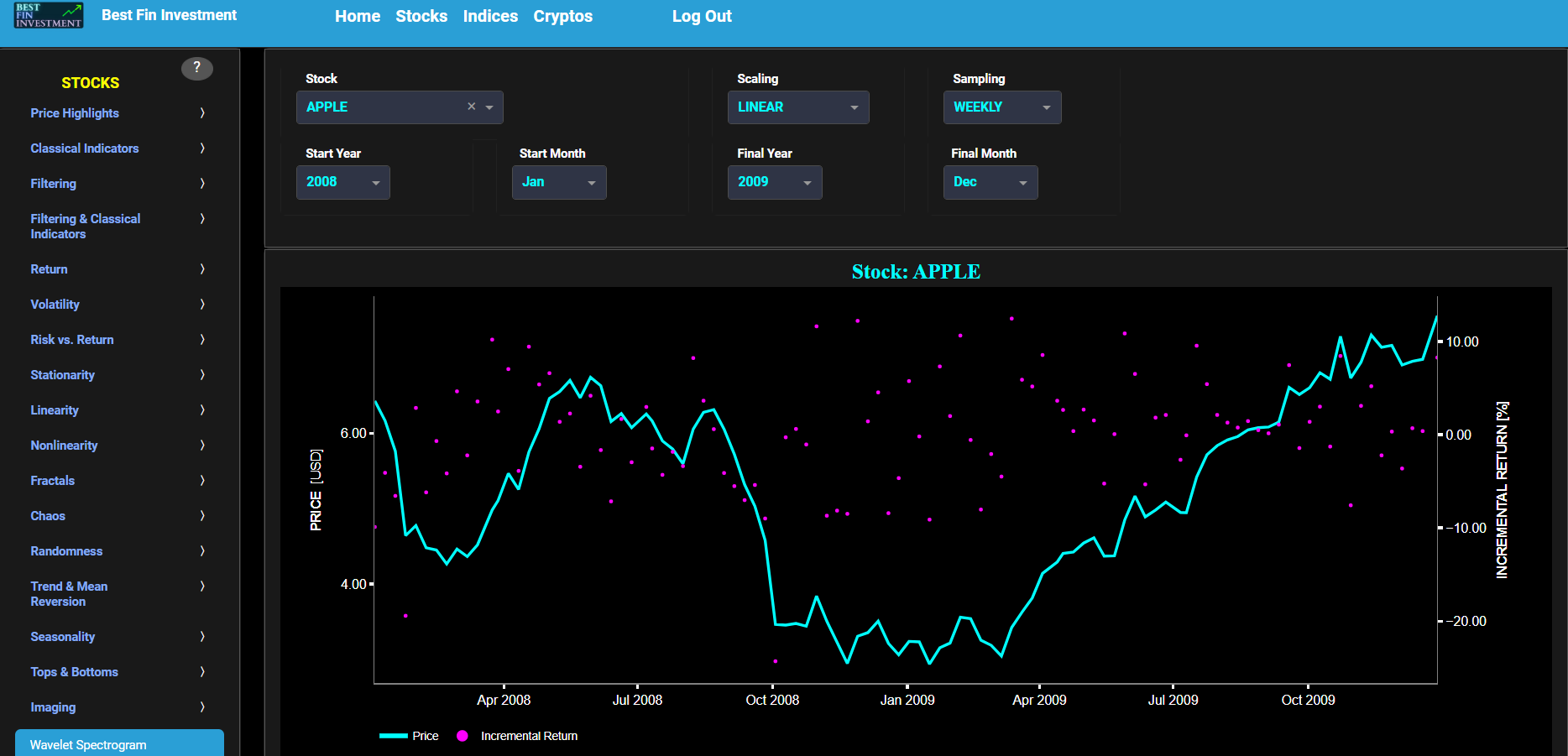
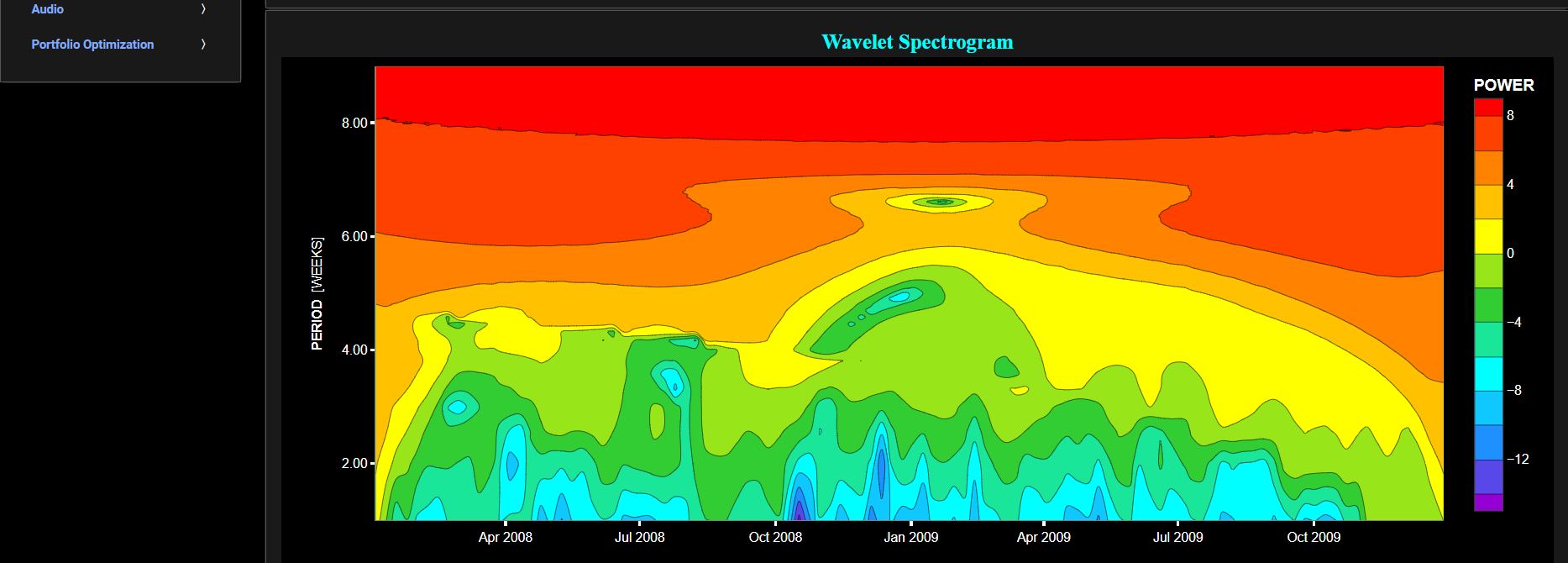
Portfolio Optimization
Risk & Return Metrics
This page provides a summary table displaying historical asset performance, including key risk and return metrics, derived from daily closing prices. You can select up to 20 assets, and for comparison, the table also includes the performance of the S&P 500. Using the menu bar above the graph, you can also customize the time periods displayed. Here the Return column is defined as the % gain or loss between the selected Start Date (Year & Month) and the Final Date (Year & Month). The Return is further shown in green for positive values and in red for negative values. The Drawdown column is a measure of the largest start-to-trough decline in the value of the financial asset, expressed as a percentage of the initial investment. Essentially, it calculates the largest percentage decrease from the Start Date (Year & Month). This column is shown in red for values below -20% and is shown in green for zero values. The volatility column shows here the annualized volatility, defined as the standard deviation of daily returns multiplied by the square root of the total number of trading days in a year, with the final result being multiplied by 100. Volatility values above 50 are shown in red, and below 50 in black. Finally the Sharpe Ratio (SR) column computes a risk-adjusted return on investment. In our case the SR is computed as the annualized return minus the risk free rate (taken here to be zero) divided by the values of the Volatility column. SR values above 1 are shown in green and SR values below 0 in red.
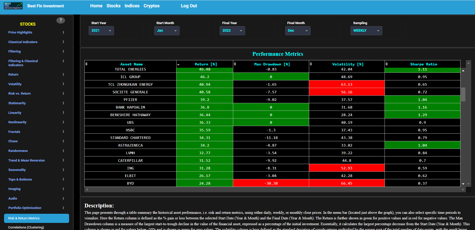
Portfolio Optimization
Correlations (Clustering)
This page provides 2 graphs. The upper graph visualizes historical asset prices in cyan color using either daily, weekly, or monthly close prices. In the menu bar (located just above the graphs), you can also select specific time periods to visualize and also toggle between a linear or logarithmic price scaling on the left y-axis. Next to the cyan line, the upper graph also visualizes the S&P500 price in magenta color (for benchmarking). Further the menu bar allows you to select one of three correlation metrics: Pearson, Spearman, and Kendall-Tau.
Once a correlation metric has been selected, the menu bar will then show the correlation value between the selected asset and the S&P500 benchmark, as well as correlation values between the selected asset and all other assets in the database. Note that the Pearson, Spearman, and Kendall-Tau correlation coefficients are all used to measure the relationship or association between pairs of variables. However, they do have distinct characteristics. The Pearson correlation coefficient measures the strength and direction of a linear relationship between two continuous variables. This metric is suitable for quantitative data that are normally distributed with constant variance (homoscedasticity). However it is rather sensitive to outliers and hence can be influenced by them. On the other hand the Spearman and Kendall-Tau correlation coefficients measure the strength and direction of a monotonic (non-linear) relationship between two variables. They are further suitable for both continuous and ordinal data, and are based upon a non-parametric approach that does not assume any specific data distribution. In addition they are much less sensitive to outliers (compared to Pearson's correlation) and are much more appropriate to variables that have a nonlinear relationship. Finally, and compared to Spearman, the Kendall's Tau metric is particularly robust when dealing with tied data points (i.e., when multiple data points have the same value).
Now the lower graph applies a clustering algorithm (i.e. a form of unsupervised learning) to all correlation coefficients that have been computed for the selected asset. First the optimal number of clusters is computed through a silhouette score, following which a tailored clustering algorithm is used to cluster the data. Next the graph produces a so-called violin plot where each cluster is represented as a separate violin, showing the distribution of correlation values within each cluster. A violin plot is a data visualization technique that combines elements of a box plot and a kernel density plot. It is particularly useful to visualize skewed distributions. Displaying clusters of correlation coefficients for an asset, i.e. by unveiling groups of assets that tend to move together or exhibit similar behavior, can provide valuable insights in various scenarios, e.g. portfolio management, risk analysis and diversification, and understanding asset relationships.

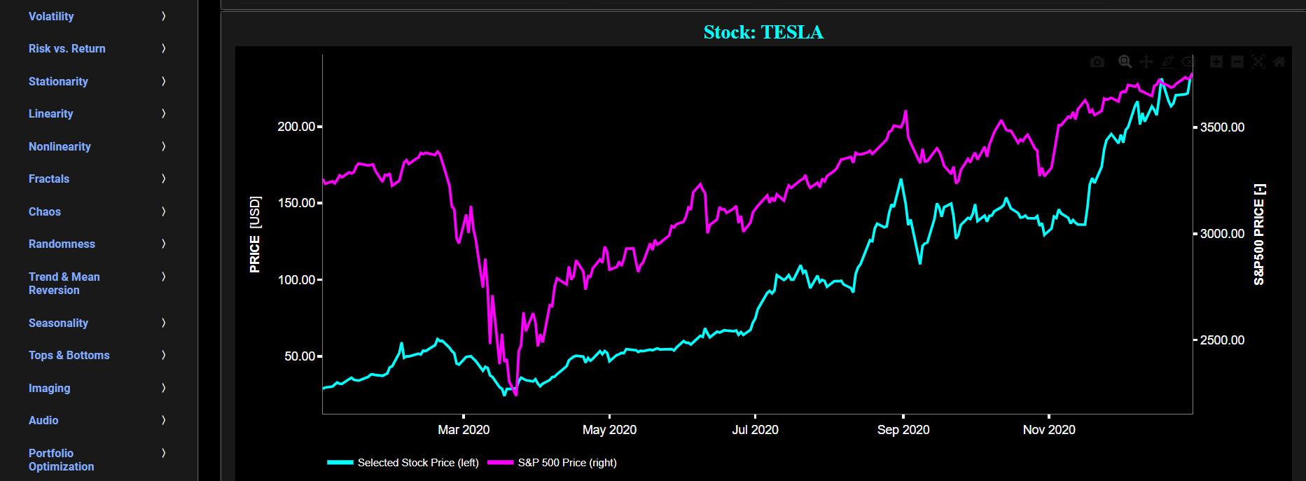
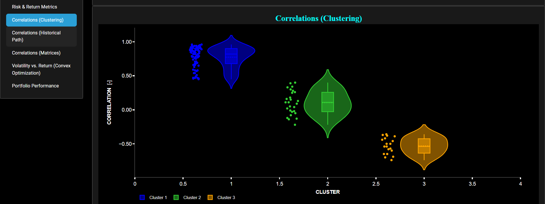
Portfolio Optimization
Correlations (Historical Path)
This page provides 2 graphs. The upper graph visualizes historical asset returns using either daily, weekly, or monthly close prices. In the menu bar (located just above the graphs), you can also select specific time periods to visualize and also toggle between a linear or logarithmic price scaling on the left y-axis. Here asset returns are defined as the % gain or loss with respect to the selected Start Date (Year & Month). The return of the reference asset is shown in cyan color. Next the return of the S&P500 is shown in magenta color (for benchmarking). In the menu bar you can also select up to 10 other assets and have their respective returns visualized in distinct colors.
Now the lower graph visualizes the historical path of the correlation coefficients between the reference asset and all other selected ones. The correlation is computed using a lookback time period that can be selected in the menu bar. Further the menu bar allows you to select one of three correlation metrics: Pearson, Spearman, and Kendall-Tau. Note that the Pearson, Spearman, and Kendall-Tau correlation coefficients are all used to measure the relationship or association between pairs of variables. However, they do have distinct characteristics. The Pearson correlation coefficient measures the strength and direction of a linear relationship between two continuous variables. This metric is suitable for quantitative data that are normally distributed with constant variance (homoscedasticity). However it is rather sensitive to outliers and hence can be influenced by them. On the other hand the Spearman and Kendall-Tau correlation coefficients measure the strength and direction of a monotonic (non-linear) relationship between two variables. They are further suitable for both continuous and ordinal data, and are based upon a non-parametric approach that does not assume any specific data distribution. In addition they are much less sensitive to outliers (compared to Pearson's correlation) and are much more appropriate to variables that have a nonlinear relationship. Finally, and compared to Spearman, the Kendall's Tau metric is particularly robust when dealing with tied data points (i.e., when multiple data points have the same value). It is clear that visualizing the historical path of correlation coefficients between a reference asset and other selected assets is a valuable tool as this provides a dynamic and informative view of how asset relationships change over time. This is essential for recognizing changing market conditions, making informed investment decisions, and managing risk effectively in a constantly evolving financial landscape.
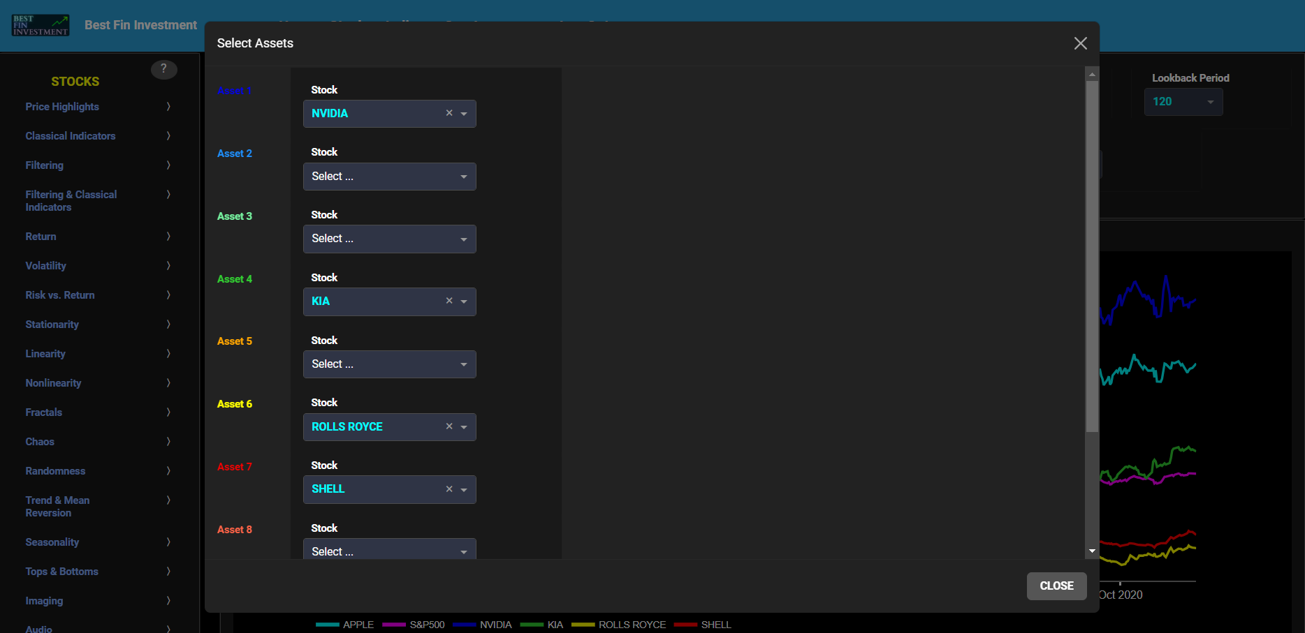
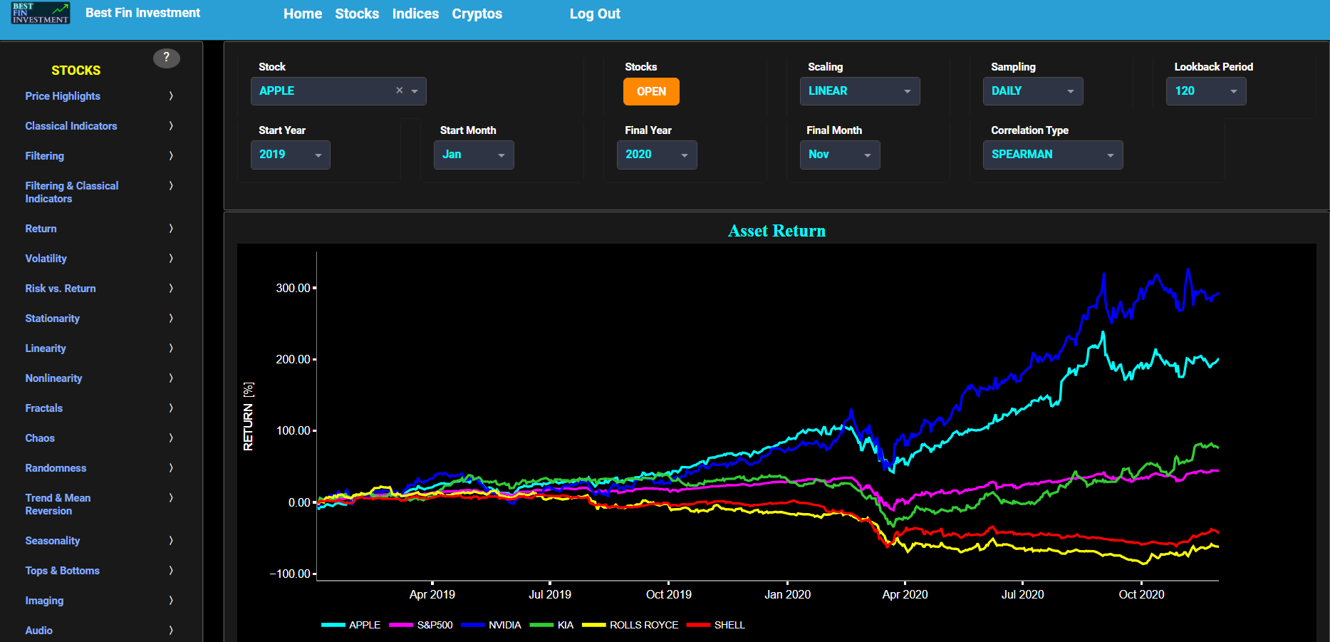
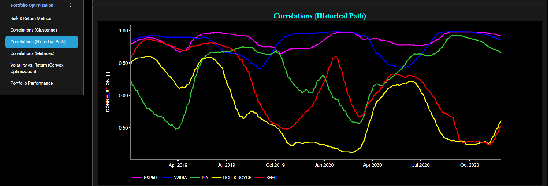
Portfolio Optimization
Correlations (Matrices)
This page provides 2 displays. The upper graph visualizes historical asset returns using either daily, weekly, or monthly close prices. In the menu bar (located just above the graphs), you can also select specific time periods to visualize and also toggle between a linear or logarithmic price scaling on the left y-axis. Here asset returns are defined as the % gain or loss with respect to the selected Start Date (Year & Month). The return of the reference asset is shown in cyan color. Next the return of the S&P500 is shown in magenta color (for benchmarking). In the menu bar you can also select up to 10 other assets and have their respective returns visualized in distinct colors.
Now the lower display presents the correlation matrix between all selected assets (including the S&P500 benchmark). The correlation coefficients are computed for the time period between the selected Start Date (Year & Month) and the Final Date (Year & Month). The cells of the correlation matrix have also been color coded: being green when the correlation moves towards -1, being white when the correlation is around 0, and being red when the correlation moves towards 1. Note that strong negative correlations (i.e. moving towards -1), indicates that the assets tend to move in opposite directions, which is a beneficial characteristic for portfolio diversification. Conversely, assets moving in tandem, or having a strong positive correlation, can be a concern. This means that when one asset's value decreases, the other tends to follow suit. From a risk perspective this means that both assets are vulnerable to similar economic and market conditions, which can lead to higher portfolio volatility and potentially larger losses.
Next the menu bar allows you to select one of three correlation metrics: Pearson, Spearman, and Kendall-Tau. Note that the Pearson, Spearman, and Kendall-Tau correlation coefficients are all used to measure the relationship or association between pairs of variables. However, they do have distinct characteristics. The Pearson correlation coefficient measures the strength and direction of a linear relationship between two continuous variables. This metric is suitable for quantitative data that are normally distributed with constant variance (homoscedasticity). However it is rather sensitive to outliers and hence can be influenced by them. On the other hand the Spearman and Kendall-Tau correlation coefficients measure the strength and direction of a monotonic (non-linear) relationship between two variables. They are further suitable for both continuous and ordinal data, and are based upon a non-parametric approach that does not assume any specific data distribution. In addition they are much less sensitive to outliers (compared to Pearson's correlation) and are much more appropriate to variables that have a nonlinear relationship. Finally, and compared to Spearman, the Kendall's Tau metric is particularly robust when dealing with tied data points (i.e., when multiple data points have the same value). In essence correlation matrices are an integral part of the so-called modern portfolio theory. These matrices play a pivotal role in making informed investment decisions and find application in several critical areas, including risk management, portfolio optimization, and asset allocation.
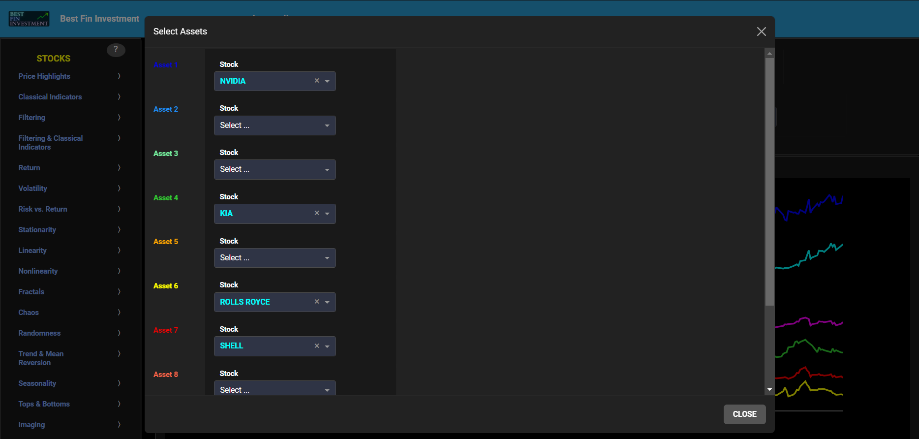
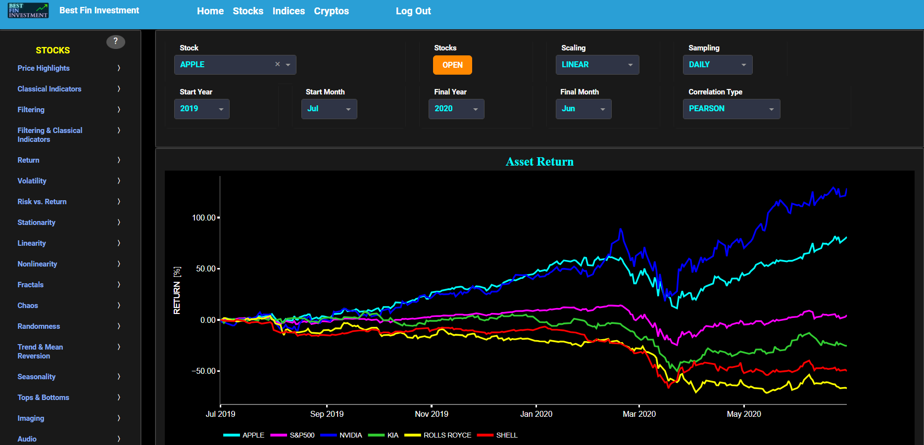
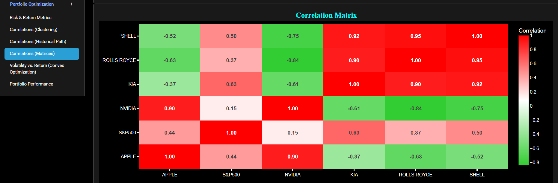
Portfolio Optimization
Volatility vs. Return (Convex Optimization)
This page provides 2 displays. The upper graph visualizes the solution space (i.e. feasible region) for a long-only portfolio optimization problem. In the menu bar (located just above the graphs), you can define the optimization problem by selecting up to 20 assets. Next you can select a specific time period and a corresponding sampling period (using either daily, weekly, or monthly close prices).
The graph plots the Pareto-optimal volatility vs. return trade-off curve (also known as the efficient frontier). Here both volatility and return are annualized metrics. The dots shown in green color lie on the efficient frontier and represent value creation portfolio’s, whereas the dots shown in red color lie on the ineficcient frontier and represent value destruction portfolio’s. The dots shown in cyan color represent sub-optimal portfolio’s. The specific asset allocation for each of these portfolio’s can be retrieved by, either, hovering the mouse above the dots or by inspecting the tables shown in the lower display. Note that this portfolio optimization problem does not take transaction costs into account. Further it is set up as a long-only portfolio optimization, meaning that the investment strategy is restricted to long positions only. In the context of investing, a "long" position involves buying an asset with the expectation that its value will increase over time, hence resulting in a profit from the price appreciation. In addition, our portfolio optimization approach is based upon historical data and is thus backward-looking in nature, in other words it determines the optimal asset allocation based upon past returns and volatilities. This means that it does not attempt to forecast or project future asset allocation; instead, it analyzes historical data to make allocation decisions for the past time period only.
Finally since our optimization problem is convex, we use a numerical optimization solver designed specifically for convex optimization problems. In particular we utilize methodologies and tools pioneered by Prof. Stephen Boyd and his research group at Stanford University to address and solve the presented portfolio optimization problem.
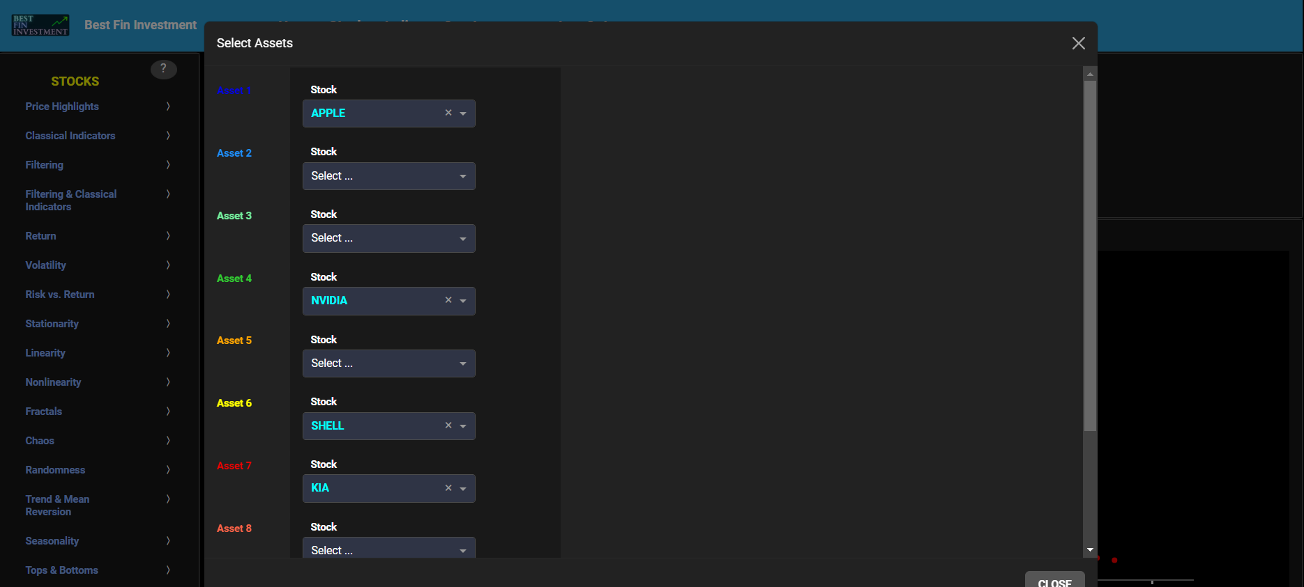
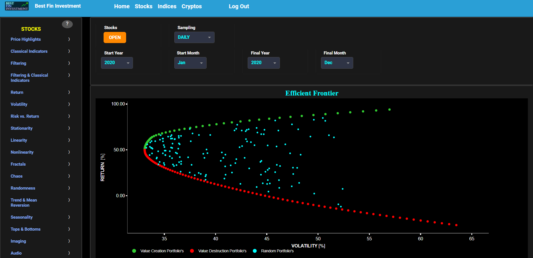
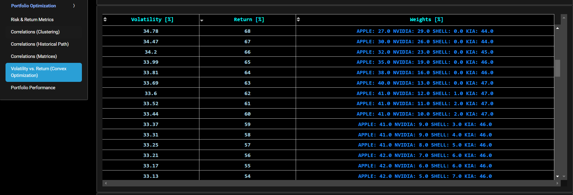
Portfolio Optimization
Portfolio Performance
This page provides 2 displays. The upper graph visualizes historical portfolio returns based upon daily close prices. In the menu bar (located just above the graph), you can also select specific time periods to visualize and select up to 3 portfolios with each portfolio having up to 20 assets. The upper graph shows also the return of the S&P500 in magenta color (for benchmarking). Here portfolio returns are defined as the % gain or loss with respect to the selected Start Date (Year & Month). The portfolio asset allocation (i.e. individual asset weight selection) may also be based upon the results shown on page “Volatility vs. Return (Convex Optimization)”.
Now the lower display presents a table summarizing the portfolio and S&P500 performance. This table is similar to the table presented on page “Risk & Return Metrics”. Here the Return column is defined as the % gain or loss between the selected Start Date (Year & Month) and the Final Date (Year & Month). The Return is further shown in green for positive values and in red for negative values. The Drawdown column is a measure of the largest start-to-trough decline in the value of the financial asset, expressed as a percentage of the initial investment. Essentially, it calculates the largest percentage decrease from the Start Date (Year & Month). This column is shown in red for values below -20% and is shown in green for zero values. The volatility column is here defined as the standard deviation of simple returns multiplied by the square root of the total number of data points, with the final result being multiplied by 100. Volatility values above 50 are shown in red, and below 50 in black. Finally the Sharpe Ratio (SR) column computes a risk-adjusted return of an investment. In our case the SR is computed as the annualized return minus the risk free rate (taken here to be zero) divided by the values of the Volatility column. SR values above 1 are shown in green and SR values below 0 in red. Overall having the ability to compare portfolio’s risk and return metrics (also against the S&P500 benchmark) helps manage risk effectively and allows to make more informed and better financial decisions.
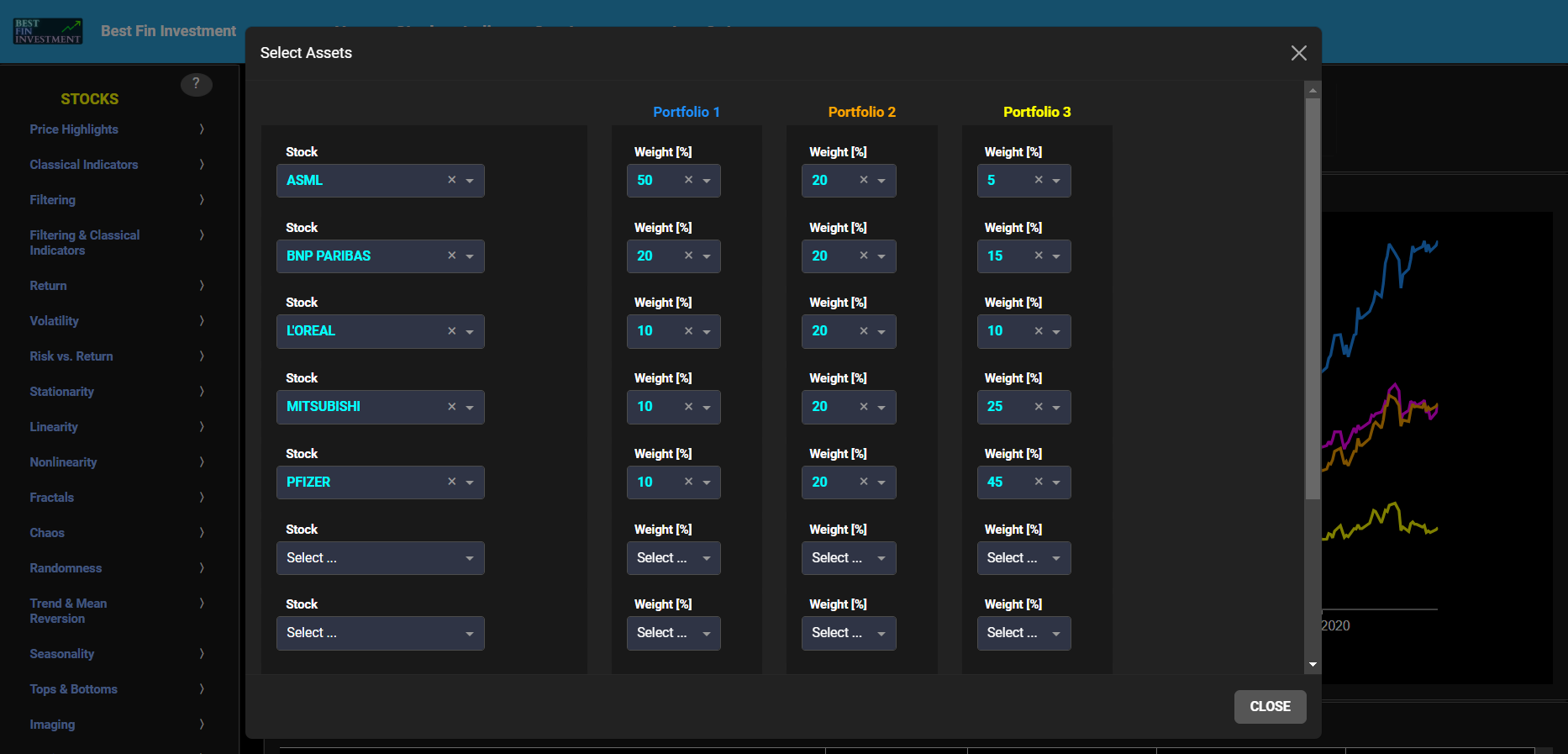
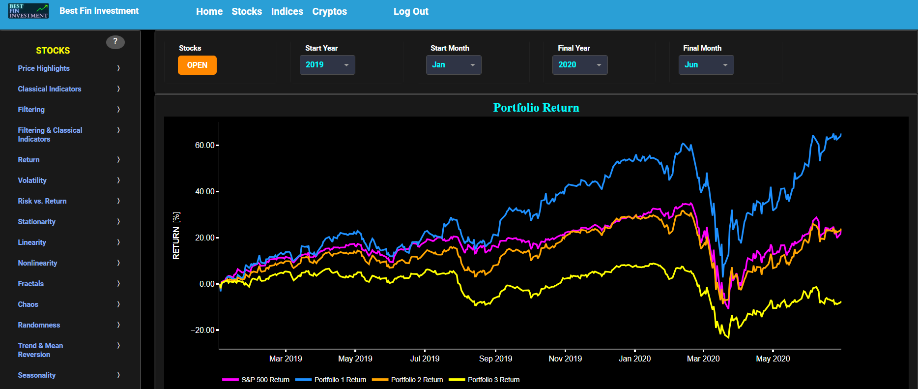
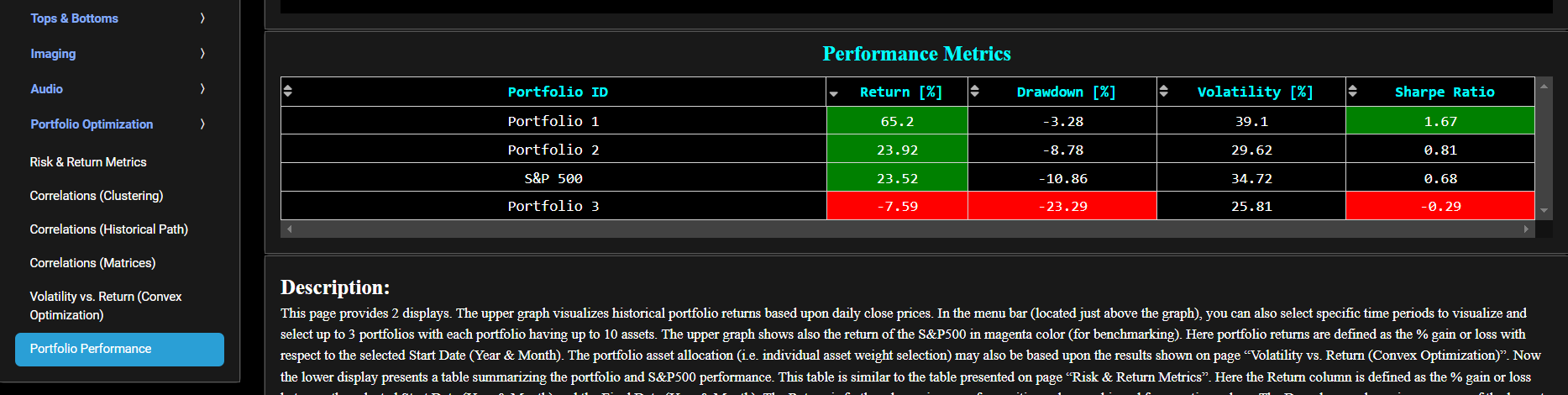
Pairs Trading
Cross Correlation Test
This page provides 3 graphs. The upper graph visualizes historical asset prices using either daily, weekly, or monthly close prices. In the menu bar (located just above the graphs), you can also select specific time periods to visualize and toggle between linear or logarithmic price scaling on the y-axis. On this graph, Asset 1 is displayed in cyan on the left y-axis, while Asset 2 is displayed in magenta on the right y-axis.
Now the middle graph displays the Pearson cross-correlation between prices of Asset 1 and Asset 2, and allows to assess the significance of this correlation using the 95% confidence interval. A positive correlation value on the y-axis means that both variables move in the same direction, whereas a negative correlation value on the y-axis means that both variables move in opposite directions. In addition, a negative lag on the x-axis (e.g. -10 units) means that changes in Asset 1 precede changes in Asset 2 by 10 time units.
Similarly the lower graph displays the Pearson cross-correlation between incremental return of Asset 1 and Asset 2, and again allows to assess the significance of this correlation using the 95% confidence interval.
Note that the cross-correlation function provides a direct measure of the linear relationship between two time series at different lags. In other words it assumes a linear relationship between the time series, which may not always hold true, and hence may not capture nonlinear relationships or time-varying dynamics.
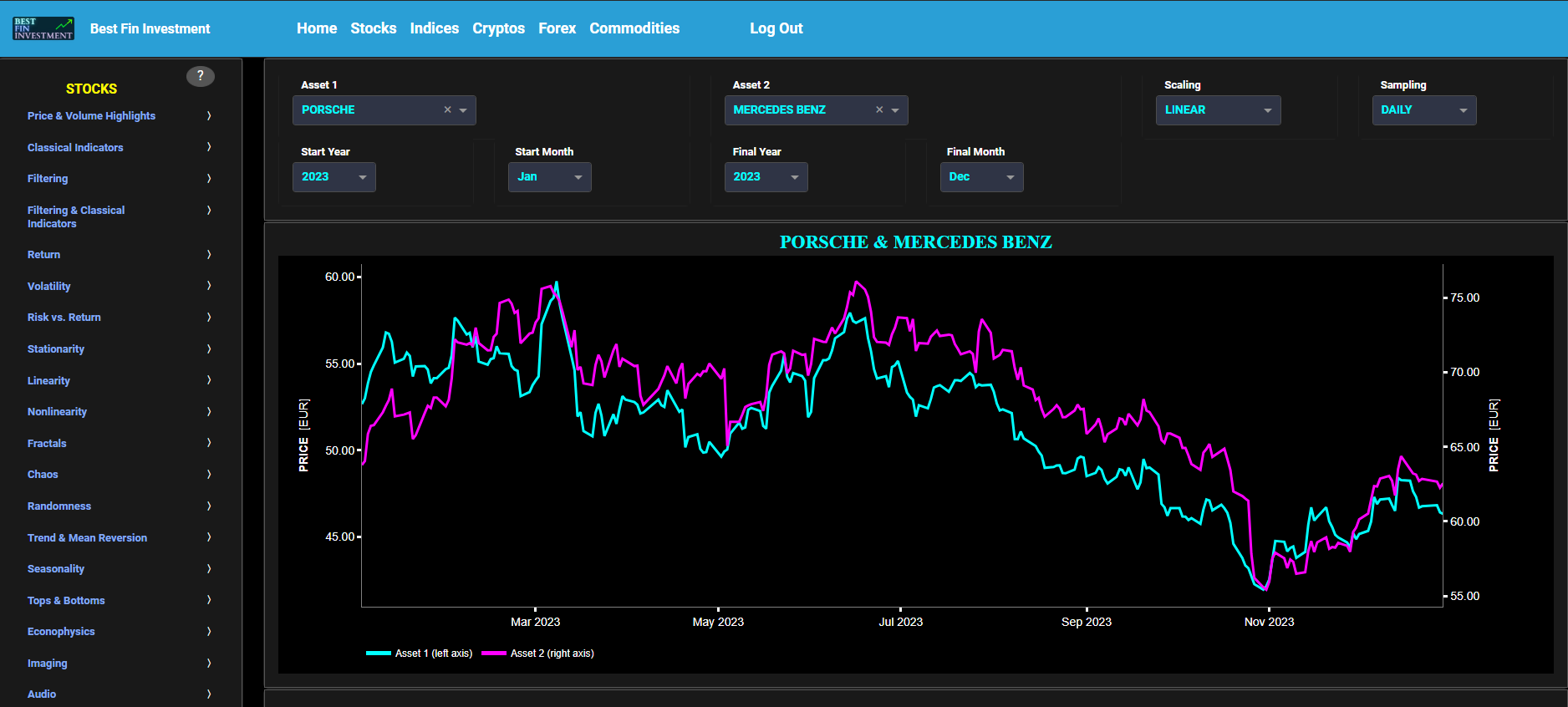
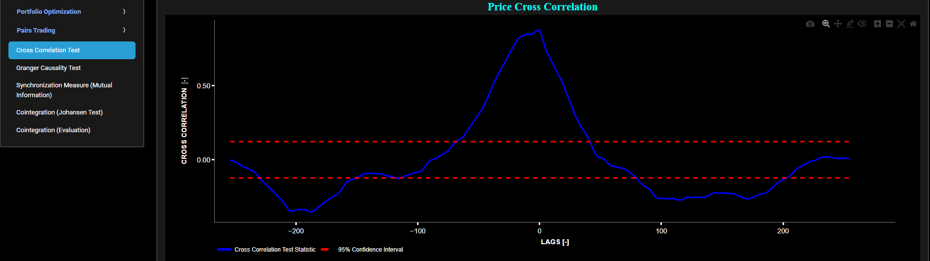
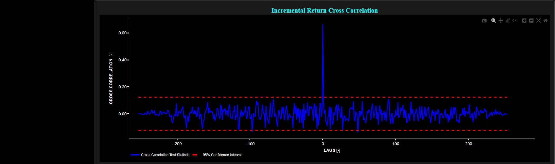
Pairs Trading
Granger Causality Test
This page provides 3 graphs. The upper graph visualizes historical asset prices using either daily, weekly, or monthly close prices. In the menu bar (located just above the graphs), you can also select specific time periods to visualize and toggle between linear or logarithmic price scaling on the y-axis. On this graph, Asset 1 is displayed in cyan on the left y-axis, while Asset 2 is displayed in magenta on the right y-axis.
Now the middle graph displays the p-value in blue color (i.e. Likelihood Ratio Test) of the Granger causality test between the price time series of Asset 1 and Asset 2 to determine if Asset 1 price has predictive power on Asset 2 price. Granger causality tests are commonly used in econometrics and time series analysis to assess whether one time series variable "Granger causes" changes in another variable. Note that the maximum number of lags for which this test is being computed can also be selected from the top menu bar.
Now if the p-value obtained from the Granger causality test is less than a chosen significance level (e.g., 0.05), it suggests that there is evidence to reject the null hypothesis that Asset 1 does not Granger cause Asset 2, hence indicating a causal relationship. Conversely, if the p-value is greater than the significance level, it suggests that there is no evidence to reject the null hypothesis, indicating no causal relationship between both Assets. Regarding the interpretation of the lag on the x-axis, suppose we observe a very low p-value at a lag of 10 units. This implies that the current changes in Asset 1 may potentially be used to predict the changes in Asset 2 that will occur in 10 time units.
The graph also shows in yellow color the p-value of the Granger causality test between Asset 1 and a benchmark signal. The latter is based upon synthetically generated, normally distributed, independent and identically distributed (i.i.d.) random signal. For this benchmark signal, each step is independent of the previous steps, and there is no systematic trend or pattern in the data. The yellow data points are given here for reference and comparison purposes (hence benchmarking).
Finally the lower graph presents the p-value in blue color of the Granger causality test between the incremental returns time series of Asset 1 and Asset 2, and in yellow color the p-value of the Granger causality test between the incremental return of Asset 1 and a synthetically generated random benchmark signal.
Note that the Granger causality test assumes linear relationships and stationary time series, and hence may produce false positives/negatives if the underlying assumptions are violated.
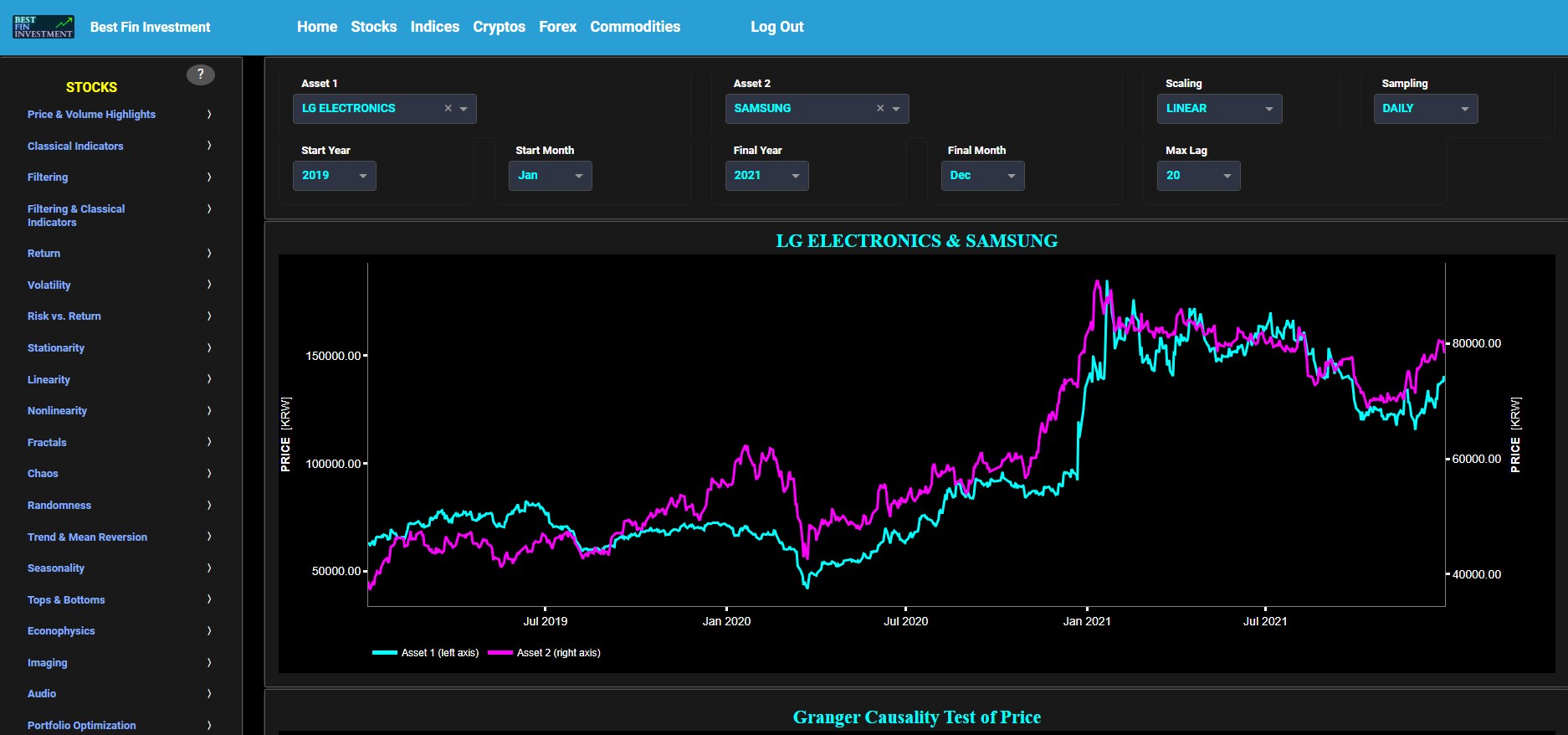
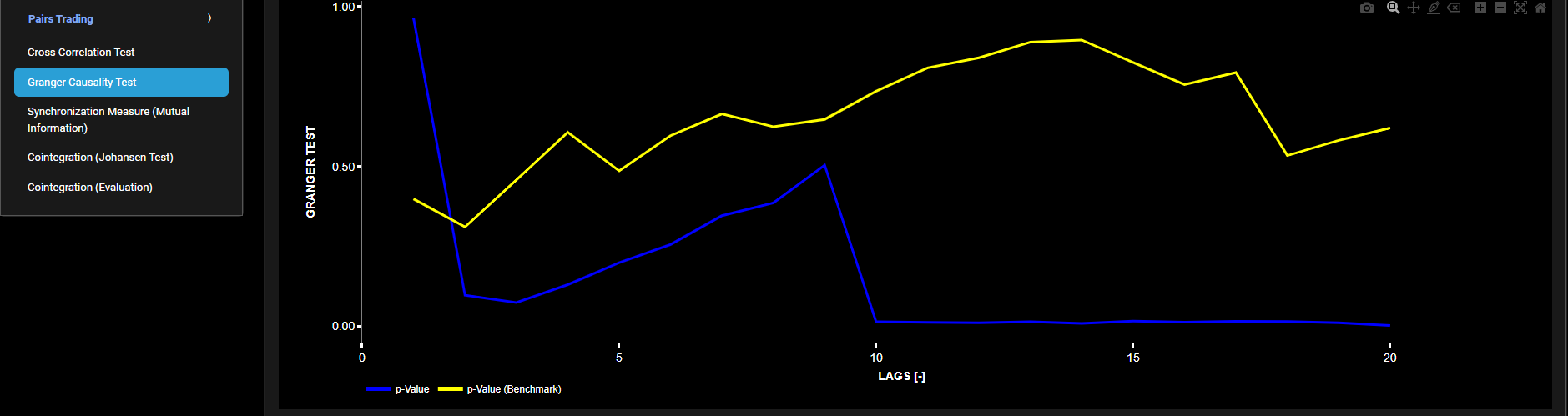
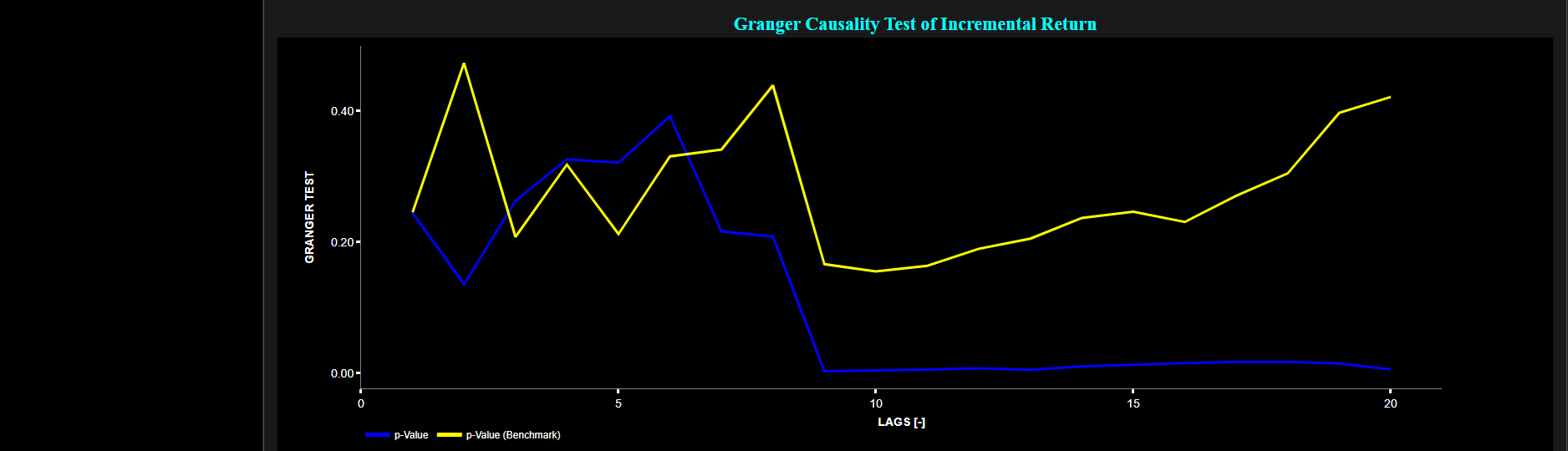
Pairs Trading
Synchronization Measure (Mutual Information)
This page provides 3 graphs. The upper graph visualizes historical asset prices using either daily, weekly, or monthly close prices. In the menu bar (located just above the graphs), you can also select specific time periods to visualize and toggle between linear or logarithmic price scaling on the y-axis. On this graph, Asset 1 is displayed in cyan on the left y-axis, while Asset 2 is displayed in magenta on the right y-axis.
The middle graph showcases the Mutual Information metric in blue, also known as a Synchronization Measure. This metric assesses the dependency between the price time series of Asset 1 and Asset 2. Mutual Information is computed for each time instant based on a user-selected lookback time period. Additionally, you can also apply a lag value to Asset 2 (selected in the top menu bar), allowing for predictions of changes in Asset 2 based on changes in Asset 1 at a specified time (i.e. lag) in the future. If for example, the lag is set to 10 units, the Mutual Information metric is computed between Asset 1 and Asset 2 shifted forward in time by 10 units. This allows for the assessment of whether changes in Asset 1 could potentially predict the changes in Asset 2 that will occur 10 time units later.
Mutual Information values indicate the degree of information shared between two time series. Higher values imply stronger dependency or predictability, while lower values suggest less dependency. A value of 0 signifies no dependency. For comparison and benchmarking, the Mutual Information metric between a synthetically generated random walk signal and Asset 2 is shown in yellow. In a random walk, each step is independent, leading to no systematic trend or pattern.
The lower graph depicts the Mutual Information metric between the incremental returns time series of Asset 1 and Asset 2 in blue. Additionally, it displays the Mutual Information metric between a synthetically generated, normally distributed, independent, and identically distributed (i.i.d.) random signal and the incremental return of Asset 2 in yellow.
It is worth noting that the Mutual Information test can identify dependencies and synchronization between time series without assuming linearity, allowing it to detect both linear and nonlinear relationships.
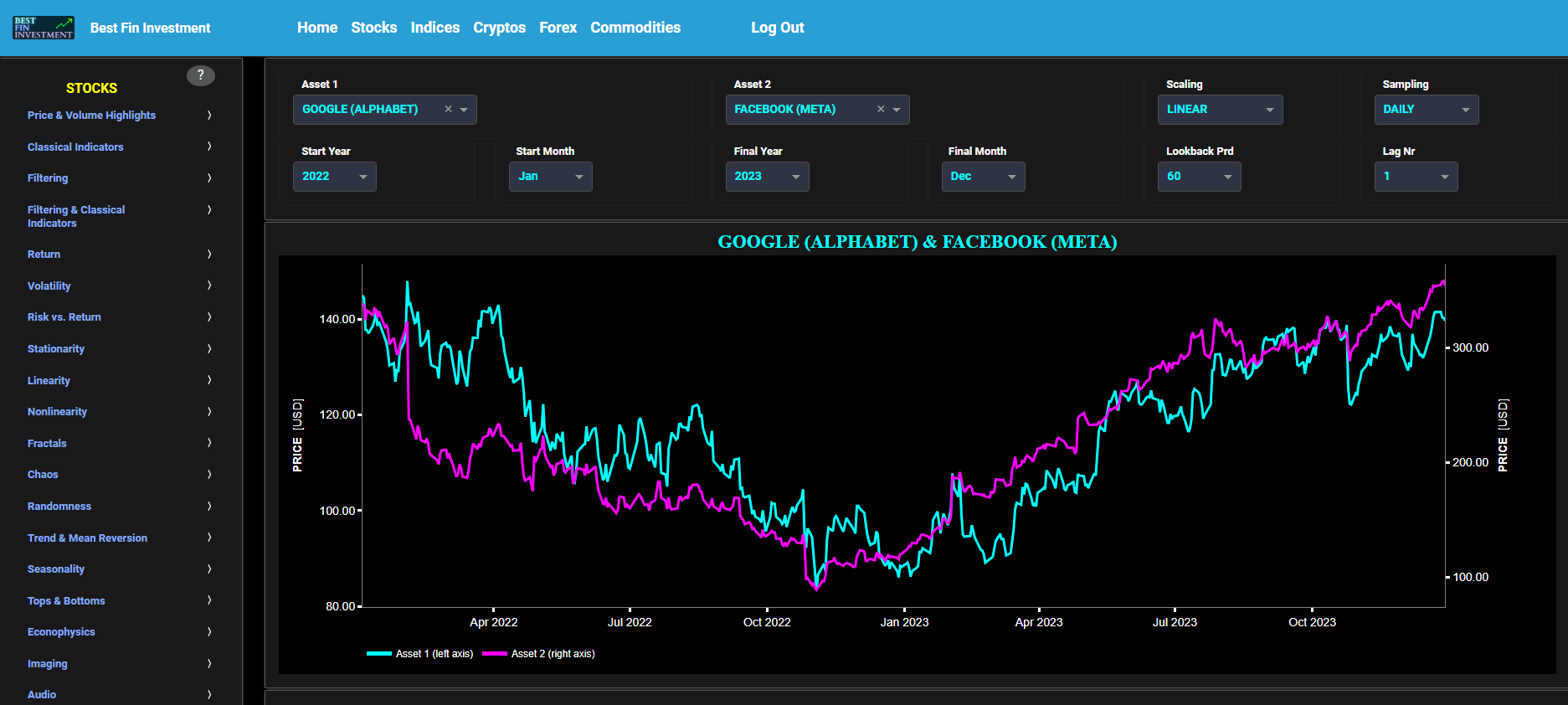
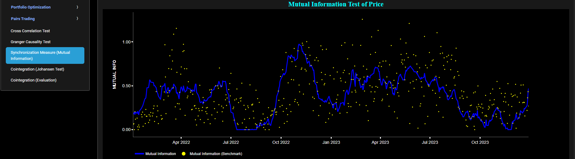
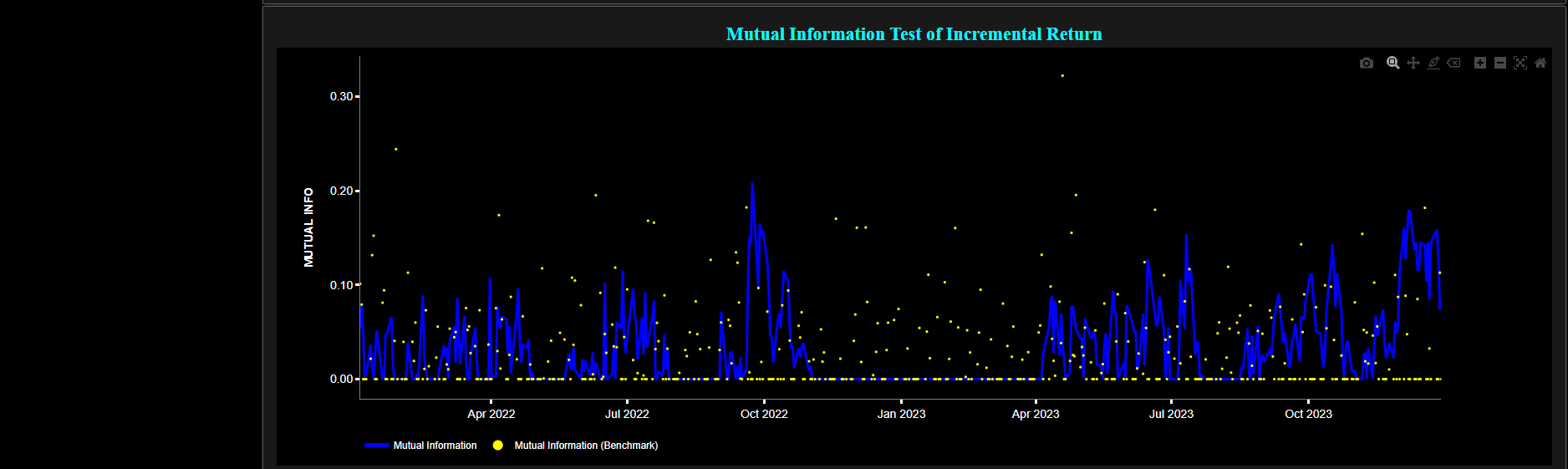
Pairs Trading
Cointegration (Johansen Test)
This page provides 4 graphs. The upper graph visualizes historical asset prices using either daily, weekly, or monthly close prices. In the menu bar (located just above the graphs), you can also select specific time periods to visualize and toggle between linear or logarithmic price scaling on the y-axis. On this graph, Asset 1 is displayed in cyan on the left y-axis, while Asset 2 is displayed in magenta on the right y-axis.
Next, we conduct a cointegration test using the Johansen method to examine the existence of a long-term equilibrium relationship between the prices of the two assets. Our objective is to determine whether the selected asset prices are cointegrated, indicating a shared stochastic trend. The Johansen test is renowned in finance for its effectiveness in identifying such long-term relationships among time series data, which can significantly influence portfolio management, risk management, and trading strategies.
The second graph illustrates the cointegrated time series in green, achieved by computing the dot product of the cointegrating vectors and the assets price data matrix. The Johansen test is here applied with the assumption of a constant term polynomial in the null-hypothesis (i.e. neglecting any time-trend). Now the cointegrating vectors are derived from the eigenvectors of the Johansen Vector Error Correction Models (VECM) coefficient matrix. Note that the Johansen test is applied on the prices of Asset 1 and Asset 2 using a lookback time period which can be selected in the top menu bar. Next the white line represents a filtered version of the cointegrated time series through the application of a low-pass Butterworth digital filter.
The third graph depicts the evolution of the cointegration coefficients, i.e. the VECM eigenvectors. The coefficient for Asset 1 is depicted in cyan, while the coefficient for Asset 2 is shown in magenta. Additionally, the graph includes filtered versions of these coefficients represented by white lines. These filtered versions are again obtained using a low-pass Butterworth digital filter.
The fourth graph displays the p-value of the Augmented Dickey-Fuller (ADF) test of the cointegrated time series in blue color on the left y-axis. Additionally, it shows the ratios of the Johansen trace statistic to the 90% and 95% critical values in orange and red colors respectively on the right y-axis.
In our case, the ADF test is applied using a constant (intercept) component when testing for the stationarity of the cointegrated time series. The null hypothesis of the ADF test posits that the time series is non-stationary, indicating it possesses a unit root. Conversely, the alternative hypothesis suggests that the time series is stationary, signifying it lacks a unit root. If the ADF p-value is less than a chosen significance level (e.g., 0.05), it is typical to reject the null hypothesis, concluding that the series is stationary. Conversely, if the p-value exceeds the significance level, we fail to reject the null hypothesis, indicating that the series is non-stationary.
Regarding the Johansen metrics depicted on the right y-axis, if the ratios exceed 1, it suggests that the computed Johansen trace statistic surpasses the critical value at the corresponding confidence level. This provides evidence for cointegration between the two price series. Conversely, if these ratios are less than or equal to 1, it indicates that the computed statistic does not surpass the critical value, suggesting no evidence of cointegration.
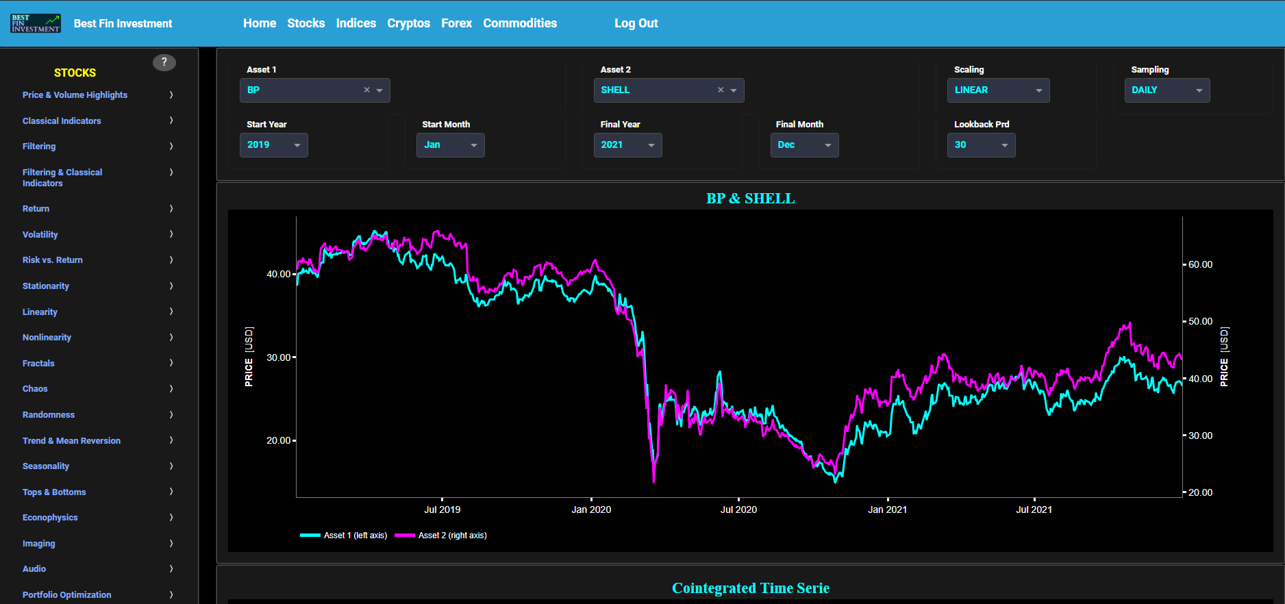
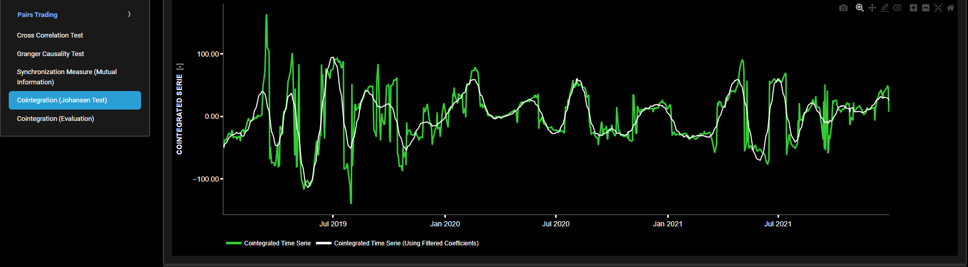
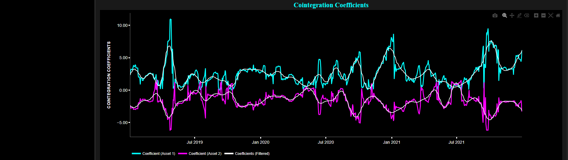
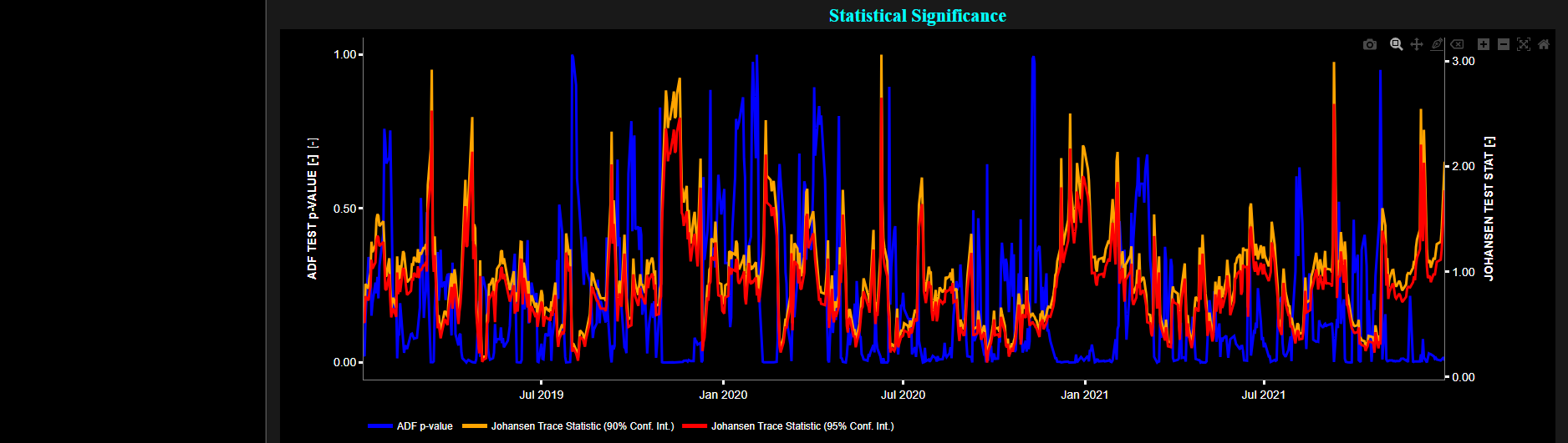
Pairs Trading
Cointegration (Evaluation)
This page provides 2 graphs. The upper graph visualizes historical asset prices using either daily, weekly, or monthly close prices. In the menu bar (located just above the graphs), you can also select specific time periods to visualize and toggle between linear or logarithmic price scaling on the y-axis. On this graph, Asset 1 is displayed in cyan on the left y-axis, while Asset 2 is displayed in magenta on the right y-axis.
Now, the lower graph displays a time series in green color on the left y-axis, referred to here as the cointegrated time series. This series is computed by combining the price series of the selected assets using the provided cointegration coefficients, which can also be selected from the top menu bar. This cointegrated time series represents the combined series of the selected assets adjusted by the provided cointegration coefficients. It is important to note that this time series may or may not exhibit cointegration.
Subsequently, this combined time series undergoes testing for stationarity using the Augmented Dickey-Fuller (ADF) test. The lower graph further presents the ADF p-value in blue color on the right y-axis. If the p-value obtained from the ADF test is less than a chosen significance level (e.g., 0.05), it indicates that the combined series is stationary, suggesting a long-term equilibrium relationship between the selected assets. Conversely, if the p-value is greater than the significance level, it suggests that the combined series is non-stationary.