Stationarity of Time Series
Blog Post by Best Fin Investment
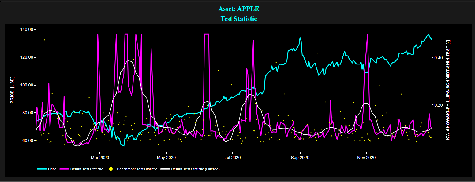
Example of Kwiatkowski–Phillips–Schmidt–Shin Test (KPSS) stationarity test for the Apple stock (using a 20-day lookback window) for January - December 2020.
Top graph: price index (cyan color), KPSS test statistic of price return (magenta color), filtered KPSS test statistic of price return (white color), and KPSS test statistic for a stationary benchmark process (yellow color).
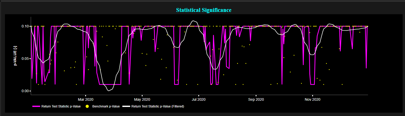
Bottom graph: statistical significance for price return (unfiltered in magenta color and filtered in white color) and for a stationary benchmark process (yellow color).
Source: Best Fin Investment Dashboard.
Table of Contents:
- Introduction
- Trend Stationarity
- Difference Stationarity
- Redefining Market Stationarity using Dr. Ernest Chan's Insight
- The Stationarity-Memory Dilemma
- Conclusion
- Explore Stationarity Metrics on the Best Fin Investment Dashboard
- References
- Related Articles
- Books from the References Section
- Additional Reads on Algorithmic Trading and Quantitative Finance
Introduction:
In its strictest sense, stationarity implies that the joint probability distribution of observations in a time series remains constant over time. For example, this means that the mean, variance, and autocovariance of a process are constant over time. Invariant processes and stationarity are often required in order to perform inferential analyses (e.g. drawing conclusions or making predictions) of financial time series [2]. This requirement is crucial for applying classical statistical tests and for deriving stable and reliable models.
Trend Stationarity:
Trend stationarity refers to a time series where the mean, variance, and autocovariance are constant over time after removing any deterministic trends. In this case, the data may exhibit a trend component, but once the trend is removed, the remaining series satisfies the criteria of stationarity.
Difference Stationarity:
Difference stationarity refers to a time series that becomes stationary after differencing, even if it is not stationary in its original form. By taking differences between consecutive observations, such as in the case of price returns, the resulting series may exhibit constant mean, variance, and autocovariance.
Redefining Market Stationarity using Dr. Ernest Chan's Insight:
From a practical perspective, Dr. Ernest Chan, a renowned author, trader, and investor, defines stationarity in financial time series as a condition where the variance of the log of prices increases more slowly than in a geometric random walk. In this context, stationarity does not imply that prices are necessarily range-bound with time-independent variance; rather, it indicates that the variance grows more slowly than typical diffusion [1]. Additionally, in this context, stationarity and mean-reversion are somewhat synonymous, characterized by a Hurst exponent H less than 0.5.
Note that the Hurst exponent H is a measure used to evaluate the long-term memory of time series data. It helps in understanding the degree of autocorrelation within the data, indicating whether the data exhibits persistence or mean-reversion. For H > 0.5, this means that the time series shows long-term positive autocorrelation, meaning that if the series has increased in the past, it is likely to continue increasing. Conversely, for H < 0.5 this means that the time series is mean-reverting, indicating that increases are likely to be followed by decreases, and vice versa.
The Stationarity-Memory Dilemma:
Stationarity is a fundamental requirement for inferential purposes. This means that for many statistical analyses and models, particularly in time series analysis (i.e. which involve drawing conclusions or making predictions based on data), the assumption that the underlying data-generating process is stationary is crucial. Indeed, if a time series is non-stationary, it may lead to misleading conclusions, as the statistical properties may change over time, affecting the reliability of the inferences made.
Therefore, when dealing with a non-stationary time series, it is common practice to apply specific data transformations to convert the original series into a stationary one.
However, these transformations, while achieving stationarity, come at the cost of erasing most or all memory from the original time series.
Memory, in this context, serves as the foundation for a model's predictive power.
Hence, a central inquiry has been articulated by Professor Lopez de Prado as follows "What is the minimum amount of differentiation that makes a price series stationary while preserving as much memory as possible?" [2]
The answer can be found in the so-called notion of "fractional differentiation".
While traditional differentiation in time series analysis involves taking integer values, such as differencing a series once (first-order differentiation) or twice (second-order differentiation) to achieve stationarity, fractional differentiation allows the degree of differencing to be a non-integer (a fraction), enabling a more nuanced transformation of the data. Note that practical implementations of fractional differentiation for stochastic processes can be found in Professor Lopez de Prado's book [2].
Conclusion:
Understanding and achieving stationarity in financial time series is essential for the robust application of statistical models and forecasting techniques. The challenge lies not only in identifying and applying the correct transformations to achieve stationarity but also in balancing this with the need to preserve the inherent memory of the data, which is crucial for predictive accuracy. The insights provided by Dr. Ernest Chan and Professor Lopez de Prado highlight the nuanced approach required to address this balance. By considering fractional differentiation, we can approach stationarity in a way that does not completely strip the data of its predictive capabilities, allowing for more sophisticated and accurate modeling of financial markets.
Explore Stationarity Metrics on the Best Fin Investment Dashboard:
- Augmented Dickey-Fuller Test
- Leybourne-McCabe Test
- Kwiatkowski–Phillips–Schmidt–Shin Test
- Phillips-Perron Test
- Zivot-Andrews Test
- Dickey-Fuller Generalized Least Squares Test
References:
[1] Chan E.P., "Algorithmic Trading: Winning Strategies and Their Rationale", Wiley, 2013.
[2] Lopez de Prado M., "Advances in Financial Machine Learning", Wiley, 2018.