Price Return: A Tale of Fat Tails
Blog Post by Best Fin Investment
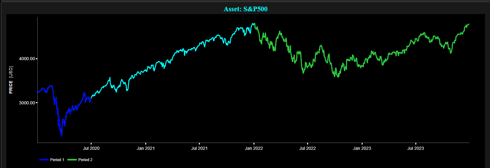
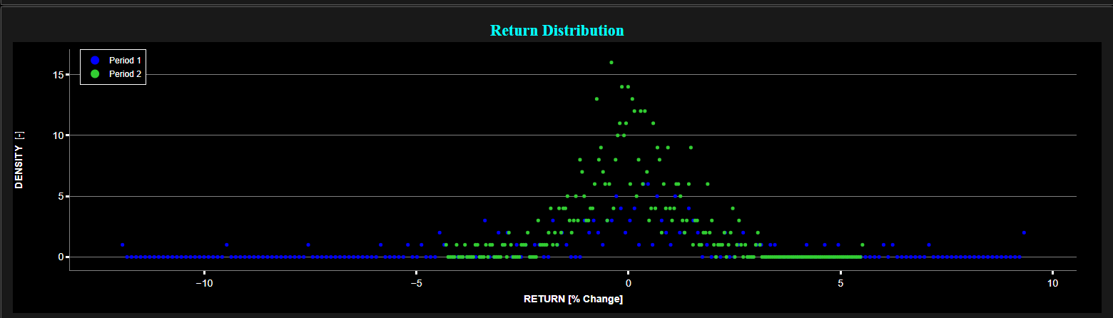
Examples of daily return distribution of the S&P 500 index.
Top graph: daily price index. Bottom graph: daily return distribution.
Time periods: January - June 2020 (blue color) and January 2022 - December 2023 (green color).
Source: Best Fin Investment Dashboard.
Table of Contents:
- Introduction
- Autocorrelations of Asset Returns
- Long-Range Memory in Autocorrelation of Nonlinear Functions of Price Return
- Fat Tails
- Price Jumps and Discontinuities
- Aggregational Gaussianity
- Time-Dependent Price Fluctuations
- Conclusion
- Explore Return Metrics on the Best Fin Investment Dashboard
- Explore Also Additional Linear Metrics on the Best Fin Investment Dashboard
- References
- Related Articles
- Books from the References Section
- Additional Reads on Human Behavior and Behavioral Finance
Introduction:
Understanding the behavior of price returns in financial markets is crucial for analysts and investors alike. In this blog post, we delve into some of the key stylized facts, i.e. nontrivial statistical properties, surrounding price returns, by shedding some light on their intriguing characteristics and potential implications.
Note that a so-called stylized fact is a feature that is consistent enough to be generally accepted as truth [9].
Autocorrelations of Asset Returns:
Asset return autocorrelation refers to the statistical relationship between an asset's past returns and its future returns. Specifically, it measures the degree to which past returns of an asset are correlated with its subsequent returns over different time intervals.
If an asset exhibits positive autocorrelation in returns, it means that if the return was positive (or negative) in the past, it is more likely to be positive (or negative) in the future.
On the other hand negative autocorrelation in returns implies that if the return was positive in the past, it is more likely to be negative in the future, and vice versa.
Finally if there is no autocorrelation in returns, the asset's past returns do not provide any predictive information about future returns. This is often associated with the concept of a "random walk" in efficient markets, where returns are deemed unpredictable. Note that high autocorrelation (be it positive or negative) in asset returns might suggest a market inefficiency, where past information is not fully reflected in the current returns, allowing for potential prediction of future returns.
For very small intraday time scales (e.g., below 20 minutes), as noted by Cont (2001) [5], evidence suggested the presence of (linear) autocorrelations in asset returns, attributed to market microstructure effects (market microstructure refers to the mechanisms that determine prices and liquidity at a granular level). However, it is important to consider that Cont's findings were contextualized in 2001 within a market structure predominantly influenced by market-makers (i.e. pre-2005). Since the advent of electronic markets in 2005, the trading landscape has been increasingly dominated by High-Frequency Trading (HFT). This shift has potentially altered the threshold at which market inefficiencies exist. With the rapid trading capabilities of HFTs, inefficiencies that once persisted up to approximately 20 minutes may now have been arbitraged away to near-zero, or to just a few seconds or a few minutes.
Similarly, at increased time scales, i.e. weekly and monthly, (linear) autocorrelations in asset returns are again observed. However, as the size of datasets is inversely proportional to time scales, the associated statistical evidence becomes less conclusive and more variable from sample to sample [5].
Now between time scales of approximately a few minutes and approximately a few weeks, the presence of (linear) autocorrelations in asset returns is generally absent [5].
Long-Range Memory in Autocorrelation of Nonlinear Functions of Price Returns:
It was shown that the autocorrelation of nonlinear functions of price returns, such as absolute returns, decays slowly as a function of the time lag (roughly as a power law) [5].
A power law decay refers to a relationship between two quantities where one quantity decreases as a power of another.
In our case this means that the autocorrelation of absolute returns will decrease slowly as the time lag quantity is increased, leading to a so-called "long tail" where even large values of the time lag still produce non-negligible autocorrelation values.
Another example includes the autocorrelation of the sign of trades which is also very long-range correlated, over several days or maybe even months [2].
Fat Tails:
Here the term "tail" refers to the tail distribution of asset returns, i.e. the behavior of the distribution of returns at the extreme ends, both in the positive and negative directions. In a probability distribution, the tails represent the areas farthest from the mean or median, where extreme values or outliers occur. In the context of asset returns, the tail distribution is concerned with the probability and magnitude of very large gains or losses, which can be critical for trading and investment strategies, risk management, and financial modeling. Interestingly this pattern of many small events and few large events is not unique to finance. It is a signature of so-called "self-organized criticality" systems [8], where other examples include earthquakes and traffic jams.
Now a so-called "fat tail" distribution in asset returns describes a situation where the tails of the distribution are thicker or "heavier" than those of a normal distribution (i.e. Gaussian distribution). This means that extreme events (both large positive and large negative returns) are more likely to occur than would be predicted by a normal distribution. Fat tails indicate greater potential for unexpected, significant changes in asset prices, hence higher trading opportunities but also higher risk.
Note also that in the literature the term "fat tails" is also typically referred to as "power law" decay, "Pareto-like tail", "long tail", "heavy tail", "non-Gaussian" character, "non-bell shape" distribution, or "excess Kurtosis". Kurtosis is defined as the fourth standardized moment of a distribution. Kurtosis measures the "peakedness" or "flatness" of a distribution relative to a normal distribution. In essence the Kurtosis quantifies the "tailedness" of a distribution, indicating how much data is in the tails compared to the rest of the distribution.
Why is it so important to understand this concept of "fat tail" distributions?
1) Because as noted by Michael J. Mauboussin the idea of an average has no meaning in a power law distribution [7].
2) Because as noted by Philip W. Anderson [1], the 1977 Nobel Prize recipient in physics: "Much of the real world is controlled as much by the 'tails' of distributions as by means or averages: by the exceptional, not the mean; by the catastrophe, not the steady drip; by the very rich, not the 'middle class'. We need to free ourselves from 'average' thinking."
Returning to asset returns, "fat tails" of price returns has been repeatedly observed in various market data, i.e. not just for stock prices, and "fat tails" are particularly pronounced for intraday data [5]. Now potential causes for these "fat tails" return distributions may include:
1) The use of leverage [10].
2) Overnight price jumps, particularly for stocks, where many of the events that most affect stock prices are released when the market is closed (e.g. obvious examples are earnings announcements that occur either after the market close or before the market open) [9].
3) The act of trading itself which impacts prices. Indeed according to [3] at least 80% of price variance is induced by self-referential effects, i.e. the lion's share of the short- to medium-term activity of financial markets is unrelated to any fundamental information or economic effects.
Finishing with a few final notes regarding return distributions, it was also shown that the shape of price return distributions was not the same at different time scales [5], and that there is also the so-called gain/loss asymmetry, particularly for stocks, where one observes large drawdowns in stock prices and stock index values but not equally large upward movements [5].
Price Jumps and Discontinuities:
Abrupt changes or discontinuities in financial markets, also known as the Noah effect [6], represent an essential ingredient of markets that helps set finance apart from the natural sciences. As pointed out by Professor B. Mandelbrot, "prices often leap and do not glide" [6].
Aggregational Gaussianity:
It has been observed that as one increases the time scale over which returns are calculated, their distributions start to look more and more like a normal distribution, i.e. bell-shape [5]. As pointed out by Professor B. Mandelbrot, the degree of "wildness" (i.e. the fatness of the tails) appears to diminish as time scales are increased towards a year or a decade [6].
Time-Dependent Price Fluctuations:
It is well known that a significant portion of price movements in financial markets tends to be concentrated within a relatively small number of time units.
For example, price changes are not uniform throughout a trading day or throughout longer time periods. Or, as Vladimir Lenin put it "there are decades in which nothing happens and weeks in which decades happen".
In his book [6], Professor B. Mandelbrot refers to the following two examples "From 1986 to 2003, the US dollar traced a long, bumpy descent against the Japanese yen. But nearly half that decline occurred on just 10 out of those 4,695 trading days. Similar statistics apply in other markets, in the 1980s, fully 40% of the positive returns from the S&P 500 index came during 10 days".
Another example is based on a quote from Professor's Burton Malkiel' book [5] in which Professor Malkiel refers to Laszlo Birinyi's book "Master Trader" as follows "Laszlo Birinyi has calculated that a buy-and-hold investor would have seen one dollar invested in the Dow Jones Industrial Average in 1900 grow to $290 by the start of 2013. Had that investor missed the best five days each year, however, that dollar investment would have been worth less than a penny in 2013."
Summarizing, price changes and market volatility tend to be unevenly distributed over time, with significant movements occurring in short bursts. Price is essentially a function of trading time, and trading time is in turn a function of clock time [6]. This clustering of large price movements can make it difficult to predict when important shifts will occur, leading to the potential for both large gains and large losses within a short period of time.
Conclusion:
The study of price returns unveils a plethora of stylized facts that characterize financial markets' dynamics. From autocorrelations aspects to the presence of heavy tails and price jumps, understanding these phenomena is essential for navigating the complexities of financial markets.
For analysts, traders and investors, recognizing these stylized facts shall help make better decisions and manage risks effectively in an ever-evolving market environment.
Explore Return Metrics on the Best Fin Investment Dashboard:
- Simple Return (Historical Observations)
- Log Return (Historical Observations)
- Distribution (Comparisons)
- Distribution (Fit)
- Distribution (Uncertainty)
- Normal Distribution Test (Kolmogorov-Smirnov)
- Normal Distribution Test (Anderson-Darling)
- Normal Distribution Test (Shapiro-Wilk)
Explore Also Additional Linear Metrics on the Best Fin Investment Dashboard:
References:
[1] Anderson P.W., "Some Thoughts About Distribution in Economics", 1977 Nobel Prize Recipient in Physics.
[2] Bouchaud J.P., "The endogenous dynamics of markets: price impact, feedback loops and instabilities", Lessons from the credit crisis, pp.345-74, 2011.
[3] Bouchaud J.P., Bonart J., Donier J., Gould M., "Trades, Quotes and Prices: Financial Markets Under the Microscope", Cambridge University Press, 2018.
[4] Cont R., "Empirical properties of asset returns: stylized facts and statistical issues", Quantitative Finance, vol. 1, issue 2, pp. 223-236, 2001.
[5] Malkiel B.G., "A Random Walk Down Wall Street: The Time-Tested Strategy for Successful Investing", W.W. Norton & Company, 2020.
[6] Mandelbrot B., Hudson R.L., "The (Mis)Behaviour of Markets: A Fractal View of Risk, Ruin and Reward", Profile Books Ltd , 2008.
[7] Mauboussin M.J., "The Success Equation: Untangling Skill and Luck in Business, Sports, and Investing", Harvard Business Review Press, 2012.
[8] Mauboussin M.J., "More Than You Know: Finding Financial Wisdom In Unconventional Places", Columbia University Press, 2013.
[9] Sinclair E., "Volatility Trading", Wiley (2nd Edition), 2013.
[10] Thurner S., Doyne Farmer J., Geanakoplos J., "Leverage causes fat tails and clustered volatility", Quantitative Finance, vol. 12, issue 5, pp. 695-707, 2012.